8.2 Hybrid Atomic Orbitals
Learning objectives.
By the end of this section, you will be able to:
- Explain the concept of atomic orbital hybridization
- Determine the hybrid orbitals associated with various molecular geometries
Thinking in terms of overlapping atomic orbitals is one way for us to explain how chemical bonds form in diatomic molecules. However, to understand how molecules with more than two atoms form stable bonds, we require a more detailed model. As an example, let us consider the water molecule, in which we have one oxygen atom bonding to two hydrogen atoms. Oxygen has the electron configuration 1 s 2 2 s 2 2 p 4 , with two unpaired electrons (one in each of the two 2 p orbitals). Valence bond theory would predict that the two O–H bonds form from the overlap of these two 2 p orbitals with the 1 s orbitals of the hydrogen atoms. If this were the case, the bond angle would be 90°, as shown in Figure 8.6 , because p orbitals are perpendicular to each other. Experimental evidence shows that the bond angle is 104.5°, not 90°. The prediction of the valence bond theory model does not match the real-world observations of a water molecule; a different model is needed.
Quantum-mechanical calculations suggest why the observed bond angles in H 2 O differ from those predicted by the overlap of the 1 s orbital of the hydrogen atoms with the 2 p orbitals of the oxygen atom. The mathematical expression known as the wave function, ψ , contains information about each orbital and the wavelike properties of electrons in an isolated atom. When atoms are bound together in a molecule, the wave functions combine to produce new mathematical descriptions that have different shapes. This process of combining the wave functions for atomic orbitals is called hybridization and is mathematically accomplished by the linear combination of atomic orbitals , LCAO, (a technique that we will encounter again later). The new orbitals that result are called hybrid orbitals . The valence orbitals in an isolated oxygen atom are a 2 s orbital and three 2 p orbitals. The valence orbitals in an oxygen atom in a water molecule differ; they consist of four equivalent hybrid orbitals that point approximately toward the corners of a tetrahedron ( Figure 8.7 ). Consequently, the overlap of the O and H orbitals should result in a tetrahedral bond angle (109.5°). The observed angle of 104.5° is experimental evidence for which quantum-mechanical calculations give a useful explanation: Valence bond theory must include a hybridization component to give accurate predictions.
The following ideas are important in understanding hybridization:
- Hybrid orbitals do not exist in isolated atoms. They are formed only in covalently bonded atoms.
- Hybrid orbitals have shapes and orientations that are very different from those of the atomic orbitals in isolated atoms.
- A set of hybrid orbitals is generated by combining atomic orbitals. The number of hybrid orbitals in a set is equal to the number of atomic orbitals that were combined to produce the set.
- All orbitals in a set of hybrid orbitals are equivalent in shape and energy.
- The type of hybrid orbitals formed in a bonded atom depends on its electron-pair geometry as predicted by the VSEPR theory.
- Hybrid orbitals overlap to form σ bonds. Unhybridized orbitals overlap to form π bonds.
In the following sections, we shall discuss the common types of hybrid orbitals.

sp Hybridization
The beryllium atom in a gaseous BeCl 2 molecule is an example of a central atom with no lone pairs of electrons in a linear arrangement of three atoms. There are two regions of valence electron density in the BeCl 2 molecule that correspond to the two covalent Be–Cl bonds. To accommodate these two electron domains, two of the Be atom’s four valence orbitals will mix to yield two hybrid orbitals. This hybridization process involves mixing of the valence s orbital with one of the valence p orbitals to yield two equivalent sp hybrid orbitals that are oriented in a linear geometry ( Figure 8.8 ). In this figure, the set of sp orbitals appears similar in shape to the original p orbital, but there is an important difference. The number of atomic orbitals combined always equals the number of hybrid orbitals formed. The p orbital is one orbital that can hold up to two electrons. The sp set is two equivalent orbitals that point 180° from each other. The two electrons that were originally in the s orbital are now distributed to the two sp orbitals, which are half filled. In gaseous BeCl 2 , these half-filled hybrid orbitals will overlap with orbitals from the chlorine atoms to form two identical σ bonds.
We illustrate the electronic differences in an isolated Be atom and in the bonded Be atom in the orbital energy-level diagram in Figure 8.9 . These diagrams represent each orbital by a horizontal line (indicating its energy) and each electron by an arrow. Energy increases toward the top of the diagram. We use one upward arrow to indicate one electron in an orbital and two arrows (up and down) to indicate two electrons of opposite spin.
When atomic orbitals hybridize, the valence electrons occupy the newly created orbitals. The Be atom had two valence electrons, so each of the sp orbitals gets one of these electrons. Each of these electrons pairs up with the unpaired electron on a chlorine atom when a hybrid orbital and a chlorine orbital overlap during the formation of the Be–Cl bonds.
Any central atom surrounded by just two regions of valence electron density in a molecule will exhibit sp hybridization. Other examples include the mercury atom in the linear HgCl 2 molecule, the zinc atom in Zn(CH 3 ) 2 , which contains a linear C–Zn–C arrangement, and the carbon atoms in HCCH and CO 2 .
Link to Learning
Check out the University of Wisconsin-Oshkosh website to learn about visualizing hybrid orbitals in three dimensions.
sp 2 Hybridization
The valence orbitals of a central atom surrounded by three regions of electron density consist of a set of three sp 2 hybrid orbitals and one unhybridized p orbital. This arrangement results from sp 2 hybridization, the mixing of one s orbital and two p orbitals to produce three identical hybrid orbitals oriented in a trigonal planar geometry ( Figure 8.10 ).
Although quantum mechanics yields the “plump” orbital lobes as depicted in Figure 8.10 , sometimes for clarity these orbitals are drawn thinner and without the minor lobes, as in Figure 8.11 , to avoid obscuring other features of a given illustration. We will use these “thinner” representations whenever the true view is too crowded to easily visualize.
The observed structure of the borane molecule, BH 3, suggests sp 2 hybridization for boron in this compound. The molecule is trigonal planar, and the boron atom is involved in three bonds to hydrogen atoms ( Figure 8.12 ). We can illustrate the comparison of orbitals and electron distribution in an isolated boron atom and in the bonded atom in BH 3 as shown in the orbital energy level diagram in Figure 8.13 . We redistribute the three valence electrons of the boron atom in the three sp 2 hybrid orbitals, and each boron electron pairs with a hydrogen electron when B–H bonds form.
Any central atom surrounded by three regions of electron density will exhibit sp 2 hybridization. This includes molecules with a lone pair on the central atom, such as ClNO ( Figure 8.14 ), or molecules with two single bonds and a double bond connected to the central atom, as in formaldehyde, CH 2 O, and ethene, H 2 CCH 2 .
sp 3 Hybridization
The valence orbitals of an atom surrounded by a tetrahedral arrangement of bonding pairs and lone pairs consist of a set of four sp 3 hybrid orbitals . The hybrids result from the mixing of one s orbital and all three p orbitals that produces four identical sp 3 hybrid orbitals ( Figure 8.15 ). Each of these hybrid orbitals points toward a different corner of a tetrahedron.
A molecule of methane, CH 4 , consists of a carbon atom surrounded by four hydrogen atoms at the corners of a tetrahedron. The carbon atom in methane exhibits sp 3 hybridization. We illustrate the orbitals and electron distribution in an isolated carbon atom and in the bonded atom in CH 4 in Figure 8.16 . The four valence electrons of the carbon atom are distributed equally in the hybrid orbitals, and each carbon electron pairs with a hydrogen electron when the C–H bonds form.
In a methane molecule, the 1 s orbital of each of the four hydrogen atoms overlaps with one of the four sp 3 orbitals of the carbon atom to form a sigma (σ) bond. This results in the formation of four strong, equivalent covalent bonds between the carbon atom and each of the hydrogen atoms to produce the methane molecule, CH 4 .
The structure of ethane, C 2 H 6, is similar to that of methane in that each carbon in ethane has four neighboring atoms arranged at the corners of a tetrahedron—three hydrogen atoms and one carbon atom ( Figure 8.17 ). However, in ethane an sp 3 orbital of one carbon atom overlaps end to end with an sp 3 orbital of a second carbon atom to form a σ bond between the two carbon atoms. Each of the remaining sp 3 hybrid orbitals overlaps with an s orbital of a hydrogen atom to form carbon–hydrogen σ bonds. The structure and overall outline of the bonding orbitals of ethane are shown in Figure 8.17 . The orientation of the two CH 3 groups is not fixed relative to each other. Experimental evidence shows that rotation around σ bonds occurs easily.
An sp 3 hybrid orbital can also hold a lone pair of electrons. For example, the nitrogen atom in ammonia is surrounded by three bonding pairs and a lone pair of electrons directed to the four corners of a tetrahedron. The nitrogen atom is sp 3 hybridized with one hybrid orbital occupied by the lone pair.
The molecular structure of water is consistent with a tetrahedral arrangement of two lone pairs and two bonding pairs of electrons. Thus we say that the oxygen atom is sp 3 hybridized, with two of the hybrid orbitals occupied by lone pairs and two by bonding pairs. Since lone pairs occupy more space than bonding pairs, structures that contain lone pairs have bond angles slightly distorted from the ideal. Perfect tetrahedra have angles of 109.5°, but the observed angles in ammonia (107.3°) and water (104.5°) are slightly smaller. Other examples of sp 3 hybridization include CCl 4 , PCl 3 , and NCl 3 .
sp 3 d and sp 3 d 2 Hybridization
To describe the five bonding orbitals in a trigonal bipyramidal arrangement, we must use five of the valence shell atomic orbitals (the s orbital, the three p orbitals, and one of the d orbitals), which gives five sp 3 d hybrid orbitals . With an octahedral arrangement of six hybrid orbitals, we must use six valence shell atomic orbitals (the s orbital, the three p orbitals, and two of the d orbitals in its valence shell), which gives six sp 3 d 2 hybrid orbitals . These hybridizations are only possible for atoms that have d orbitals in their valence subshells (that is, not those in the first or second period).
In a molecule of phosphorus pentachloride, PCl 5 , there are five P–Cl bonds (thus five pairs of valence electrons around the phosphorus atom) directed toward the corners of a trigonal bipyramid. We use the 3 s orbital, the three 3 p orbitals, and one of the 3 d orbitals to form the set of five sp 3 d hybrid orbitals ( Figure 8.19 ) that are involved in the P–Cl bonds. Other atoms that exhibit sp 3 d hybridization include the sulfur atom in SF 4 and the chlorine atoms in ClF 3 and in ClF 4 + . ClF 4 + . (The electrons on fluorine atoms are omitted for clarity.)
The sulfur atom in sulfur hexafluoride, SF 6 , exhibits sp 3 d 2 hybridization. A molecule of sulfur hexafluoride has six bonding pairs of electrons connecting six fluorine atoms to a single sulfur atom. There are no lone pairs of electrons on the central atom. To bond six fluorine atoms, the 3 s orbital, the three 3 p orbitals, and two of the 3 d orbitals form six equivalent sp 3 d 2 hybrid orbitals, each directed toward a different corner of an octahedron. Other atoms that exhibit sp 3 d 2 hybridization include the phosphorus atom in PCl 6 − , PCl 6 − , the iodine atom in the interhalogens IF 6 + , IF 6 + , IF 5 , ICl 4 − , ICl 4 − , IF 4 − IF 4 − and the xenon atom in XeF 4 .
Assignment of Hybrid Orbitals to Central Atoms
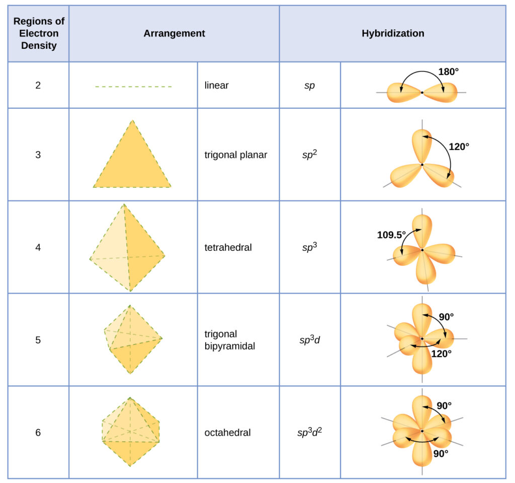
The hybridization of an atom is determined based on the number of regions of electron density that surround it. The geometrical arrangements characteristic of the various sets of hybrid orbitals are shown in Figure 8.21 . These arrangements are identical to those of the electron-pair geometries predicted by VSEPR theory. VSEPR theory predicts the shapes of molecules, and hybrid orbital theory provides an explanation for how those shapes are formed. To find the hybridization of a central atom, we can use the following guidelines:
- Determine the Lewis structure of the molecule.
- Determine the number of regions of electron density around an atom using VSEPR theory, in which single bonds, multiple bonds, radicals, and lone pairs each count as one region.
- Assign the set of hybridized orbitals from Figure 8.21 that corresponds to this geometry.
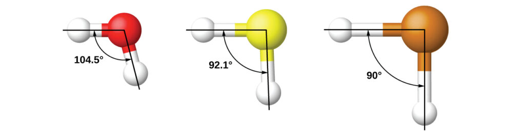
It is important to remember that hybridization was devised to rationalize experimentally observed molecular geometries. The model works well for molecules containing small central atoms, in which the valence electron pairs are close together in space. However, for larger central atoms, the valence-shell electron pairs are farther from the nucleus, and there are fewer repulsions. Their compounds exhibit structures that are often not consistent with VSEPR theory, and hybridized orbitals are not necessary to explain the observed data. For example, we have discussed the H–O–H bond angle in H 2 O, 104.5°, which is more consistent with sp 3 hybrid orbitals (109.5°) on the central atom than with 2 p orbitals (90°). Sulfur is in the same group as oxygen, and H 2 S has a similar Lewis structure. However, it has a much smaller bond angle (92.1°), which indicates much less hybridization on sulfur than oxygen. Continuing down the group, tellurium is even larger than sulfur, and for H 2 Te, the observed bond angle (90°) is consistent with overlap of the 5 p orbitals, without invoking hybridization. We invoke hybridization where it is necessary to explain the observed structures.
Example 8.2
Assigning hybridization, check your learning.
The selenium atom is sp 3 d hybridized.
Example 8.3
The carbon atom is surrounded by three regions of electron density, positioned in a trigonal planar arrangement. The hybridization in a trigonal planar electron pair geometry is sp 2 ( Figure 8.21 ), which is the hybridization of the carbon atom in urea.
H 3 C , sp 3 ; C (O)OH, sp 2
- 1 Note that orbitals may sometimes be drawn in an elongated “balloon” shape rather than in a more realistic “plump” shape in order to make the geometry easier to visualize.
As an Amazon Associate we earn from qualifying purchases.
This book may not be used in the training of large language models or otherwise be ingested into large language models or generative AI offerings without OpenStax's permission.
Want to cite, share, or modify this book? This book uses the Creative Commons Attribution License and you must attribute OpenStax.
Access for free at https://openstax.org/books/chemistry-2e/pages/1-introduction
- Authors: Paul Flowers, Klaus Theopold, Richard Langley, William R. Robinson, PhD
- Publisher/website: OpenStax
- Book title: Chemistry 2e
- Publication date: Feb 14, 2019
- Location: Houston, Texas
- Book URL: https://openstax.org/books/chemistry-2e/pages/1-introduction
- Section URL: https://openstax.org/books/chemistry-2e/pages/8-2-hybrid-atomic-orbitals
© Jan 8, 2024 OpenStax. Textbook content produced by OpenStax is licensed under a Creative Commons Attribution License . The OpenStax name, OpenStax logo, OpenStax book covers, OpenStax CNX name, and OpenStax CNX logo are not subject to the Creative Commons license and may not be reproduced without the prior and express written consent of Rice University.
Chapter 8: Advanced Theories of Covalent Bonding
8.2 hybrid atomic orbitals.
Learning Objectives
By the end of this section, you will be able to:
- Explain the concept of atomic orbital hybridization
- Determine the hybrid orbitals associated with various molecular geometries

Figure 1. The hypothetical overlap of two of the 2 p orbitals on an oxygen atom (red) with the 1s orbitals of two hydrogen atoms (blue) would produce a bond angle of 90°. This is not consistent with experimental evidence.
Thinking in terms of overlapping atomic orbitals is one way for us to explain how chemical bonds form in diatomic molecules. However, to understand how molecules with more than two atoms form stable bonds, we require a more detailed model. As an example, let us consider the water molecule, in which we have one oxygen atom bonding to two hydrogen atoms. Oxygen has the electron configuration 1 s 2 2 s 2 2 p 4 , with two unpaired electrons (one in each of the two 2p orbitals). Valence bond theory would predict that the two O–H bonds form from the overlap of these two 2 p orbitals with the 1 s orbitals of the hydrogen atoms. If this were the case, the bond angle would be 90°, as shown in Figure 1, because p orbitals are perpendicular to each other.
Experimental evidence shows that the bond angle is 104.5°, not 90°. The prediction of the valence bond theory model does not match the real-world observations of a water molecule; a different model is needed. Quantum-mechanical calculations suggest why the observed bond angles in H 2 O differ from those predicted by the overlap of the 1 s orbital of the hydrogen atoms with the 2 p orbitals of the oxygen atom. The mathematical expression known as the wave function, ψ , contains information about each orbital and the wavelike properties of electrons in an isolated atom. When atoms are bound together in a molecule, the wave functions combine to produce new mathematical descriptions that have different shapes. This process of combining the wave functions for atomic orbitals is called hybridization and is mathematically accomplished by the linear combination of atomic orbitals , LCAO, (a technique that we will encounter again later). The new orbitals that result are called hybrid orbitals . The valence orbitals in an isolated oxygen atom are a 2 s orbital and three 2 p orbitals. The valence orbitals in an oxygen atom in a water molecule differ; they consist of four equivalent hybrid orbitals that point approximately toward the corners of a tetrahedron (Figure 2). Consequently, the overlap of the O and H orbitals should result in a tetrahedral bond angle (109.5°). The observed angle of 104.5° is experimental evidence for which quantum-mechanical calculations give a useful explanation: Valence bond theory must include a hybridization component to give accurate predictions.

Figure 2. (a) A water molecule has four regions of electron density, so VSEPR theory predicts a tetrahedral arrangement of hybrid orbitals. (b) Two of the hybrid orbitals on oxygen contain lone pairs, and the other two overlap with the 1 s orbitals of hydrogen atoms to form the O–H bonds in H 2 O. This description is more consistent with the experimental structure.
The following ideas are important in understanding hybridization:
- Hybrid orbitals do not exist in isolated atoms. They are formed only in covalently bonded atoms.
- Hybrid orbitals have shapes and orientations that are very different from those of the atomic orbitals in isolated atoms.
- A set of hybrid orbitals is generated by combining atomic orbitals. The number of hybrid orbitals in a set is equal to the number of atomic orbitals that were combined to produce the set.
- All orbitals in a set of hybrid orbitals are equivalent in shape and energy.
- The type of hybrid orbitals formed in a bonded atom depends on its electron-pair geometry as predicted by the VSEPR theory.
- Hybrid orbitals overlap to form σ bonds. Unhybridized orbitals overlap to form π bonds.
In the following sections, we shall discuss the common types of hybrid orbitals.
sp Hybridization
The beryllium atom in a gaseous BeCl 2 molecule is an example of a central atom with no lone pairs of electrons in a linear arrangement of three atoms. There are two regions of valence electron density in the BeCl 2 molecule that correspond to the two covalent Be–Cl bonds. To accommodate these two electron domains, two of the Be atom’s four valence orbitals will mix to yield two hybrid orbitals. This hybridization process involves mixing of the valence s orbital with one of the valence p orbitals to yield two equivalent sp hybrid orbitals that are oriented in a linear geometry (Figure 3). In this figure, the set of sp orbitals appears similar in shape to the original p orbital, but there is an important difference. The number of atomic orbitals combined always equals the number of hybrid orbitals formed. The p orbital is one orbital that can hold up to two electrons. The sp set is two equivalent orbitals that point 180° from each other. The two electrons that were originally in the s orbital are now distributed to the two sp orbitals, which are half filled. In gaseous BeCl 2 , these half-filled hybrid orbitals will overlap with orbitals from the chlorine atoms to form two identical σ bonds.

Figure 3. Hybridization of an s orbital (blue) and a p orbital (red) of the same atom produces two sp hybrid orbitals (purple). Each hybrid orbital is oriented primarily in just one direction. Note that each sp orbital contains one lobe that is significantly larger than the other. The set of two sp orbitals are oriented at 180°, which is consistent with the geometry for two domains.
We illustrate the electronic differences in an isolated Be atom and in the bonded Be atom in the orbital energy-level diagram in Figure 4. These diagrams represent each orbital by a horizontal line (indicating its energy) and each electron by an arrow. Energy increases toward the top of the diagram. We use one upward arrow to indicate one electron in an orbital and two arrows (up and down) to indicate two electrons of opposite spin.

Figure 4. This orbital energy-level diagram shows the sp hybridized orbitals on Be in the linear BeCl 2 molecule. Each of the two sp hybrid orbitals holds one electron and is thus half filled and available for bonding via overlap with a Cl 3 p orbital.
When atomic orbitals hybridize, the valence electrons occupy the newly created orbitals. The Be atom had two valence electrons, so each of the sp orbitals gets one of these electrons. Each of these electrons pairs up with the unpaired electron on a chlorine atom when a hybrid orbital and a chlorine orbital overlap during the formation of the Be–Cl bonds. Any central atom surrounded by just two regions of valence electron density in a molecule will exhibit sp hybridization. Other examples include the mercury atom in the linear HgCl 2 molecule, the zinc atom in Zn(CH 3 ) 2 , which contains a linear C–Zn–C arrangement, and the carbon atoms in HCCH and CO 2 .
sp 2 Hybridization
The valence orbitals of a central atom surrounded by three regions of electron density consist of a set of three sp 2 hybrid orbitals and one unhybridized p orbital. This arrangement results from sp 2 hybridization, the mixing of one s orbital and two p orbitals to produce three identical hybrid orbitals oriented in a trigonal planar geometry (Figure 5).

Figure 5. The hybridization of an s orbital (blue) and two p orbitals (red) produces three equivalent sp 2 hybridized orbitals (purple) oriented at 120° with respect to each other. The remaining unhybridized p orbital is not shown here, but is located along the z axis.

Figure 6. This alternate way of drawing the trigonal planar sp 2 hybrid orbitals is sometimes used in more crowded figures.
Although quantum mechanics yields the “plump” orbital lobes as depicted in Figure 5, sometimes for clarity these orbitals are drawn thinner and without the minor lobes, as in Figure 6, to avoid obscuring other features of a given illustration.
We will use these “thinner” representations whenever the true view is too crowded to easily visualize.The observed structure of the borane molecule, BH 3 , suggests sp 2 hybridization for boron in this compound. The molecule is trigonal planar, and the boron atom is involved in three bonds to hydrogen atoms (Figure 7).

Figure 7. BH 3 is an electron-deficient molecule with a trigonal planar structure.
We can illustrate the comparison of orbitals and electron distribution in an isolated boron atom and in the bonded atom in BH 3 as shown in the orbital energy level diagram in Figure 8. We redistribute the three valence electrons of the boron atom in the three sp 2 hybrid orbitals, and each boron electron pairs with a hydrogen electron when B–H bonds form.

Figure 8. In an isolated B atom, there are one 2 s and three 2 p valence orbitals. When boron is in a molecule with three regions of electron density, three of the orbitals hybridize and create a set of three sp 2 orbitals and one unhybridized 2 p orbital. The three half-filled hybrid orbitals each overlap with an orbital from a hydrogen atom to form three σ bonds in BH 3 .
Any central atom surrounded by three regions of electron density will exhibit sp 2 hybridization. This includes molecules with a lone pair on the central atom, such as ClNO (Figure 9), or molecules with two single bonds and a double bond connected to the central atom, as in formaldehyde, CH 2 O, and ethene, H 2 CCH 2 .

Figure 9. The central atom(s) in each of the structures shown contain three regions of electron density and are sp 2 hybridized. As we know from the discussion of VSEPR theory, a region of electron density contains all of the electrons that point in one direction. A lone pair, an unpaired electron, a single bond, or a multiple bond would each count as one region of electron density.
sp 3 Hybridization
The valence orbitals of an atom surrounded by a tetrahedral arrangement of bonding pairs and lone pairs consist of a set of four sp 3 hybrid orbitals . The hybrids result from the mixing of one s orbital and all three p orbitals that produces four identical sp 3 hybrid orbitals (Figure 10). Each of these hybrid orbitals points toward a different corner of a tetrahedron.

Figure 10. The hybridization of an s orbital (blue) and three p orbitals (red) produces four equivalent sp 3 hybridized orbitals (purple) oriented at 109.5° with respect to each other.
A molecule of methane, CH 4 , consists of a carbon atom surrounded by four hydrogen atoms at the corners of a tetrahedron. The carbon atom in methane exhibits sp 3 hybridization. We illustrate the orbitals and electron distribution in an isolated carbon atom and in the bonded atom in CH 4 in Figure 11. The four valence electrons of the carbon atom are distributed equally in the hybrid orbitals, and each carbon electron pairs with a hydrogen electron when the C–H bonds form.

Figure 11. The four valence atomic orbitals from an isolated carbon atom all hybridize when the carbon bonds in a molecule like CH 4 with four regions of electron density. This creates four equivalent sp 3 hybridized orbitals. Overlap of each of the hybrid orbitals with a hydrogen orbital creates a C–H σ bond.
In a methane molecule, the 1 s orbital of each of the four hydrogen atoms overlaps with one of the four sp 3 orbitals of the carbon atom to form a sigma (σ) bond. This results in the formation of four strong, equivalent covalent bonds between the carbon atom and each of the hydrogen atoms to produce the methane molecule, CH 4 . The structure of ethane, C 2 H 6, is similar to that of methane in that each carbon in ethane has four neighboring atoms arranged at the corners of a tetrahedron—three hydrogen atoms and one carbon atom (Figure 12). However, in ethane an sp 3 orbital of one carbon atom overlaps end to end with an sp 3 orbital of a second carbon atom to form a σ bond between the two carbon atoms. Each of the remaining sp 3 hybrid orbitals overlaps with an s orbital of a hydrogen atom to form carbon–hydrogen σ bonds. The structure and overall outline of the bonding orbitals of ethane are shown in Figure 12. The orientation of the two CH 3 groups is not fixed relative to each other. Experimental evidence shows that rotation around σ bonds occurs easily.

Figure 12. (a) In the ethane molecule, C 2 H 6 , each carbon has four sp 3 orbitals. (b) These four orbitals overlap to form seven σ bonds.
An sp 3 hybrid orbital can also hold a lone pair of electrons. For example, the nitrogen atom in ammonia is surrounded by three bonding pairs and a lone pair of electrons directed to the four corners of a tetrahedron. The nitrogen atom is sp 3 hybridized with one hybrid orbital occupied by the lone pair. The molecular structure of water is consistent with a tetrahedral arrangement of two lone pairs and two bonding pairs of electrons. Thus we say that the oxygen atom is sp 3 hybridized, with two of the hybrid orbitals occupied by lone pairs and two by bonding pairs. Since lone pairs occupy more space than bonding pairs, structures that contain lone pairs have bond angles slightly distorted from the ideal. Perfect tetrahedra have angles of 109.5°, but the observed angles in ammonia (107.3°) and water (104.5°) are slightly smaller. Other examples of sp 3 hybridization include CCl 4 , PCl 3 , and NCl 3 .
sp 3 d and sp 3 d 2 Hybridization
To describe the five bonding orbitals in a trigonal bipyramidal arrangement, we must use five of the valence shell atomic orbitals (the s orbital, the three p orbitals, and one of the d orbitals), which gives five sp 3 d hybrid orbitals . With an octahedral arrangement of six hybrid orbitals, we must use six valence shell atomic orbitals (the s orbital, the three p orbitals, and two of the d orbitals in its valence shell), which gives six sp 3 d 2 hybrid orbitals . These hybridizations are only possible for atoms that have d orbitals in their valence subshells (that is, not those in the first or second period). In a molecule of phosphorus pentachloride, PCl 5 , there are five P–Cl bonds (thus five pairs of valence electrons around the phosphorus atom) directed toward the corners of a trigonal bipyramid. We use the 3 s orbital, the three 3 p orbitals, and one of the 3 d orbitals to form the set of five sp 3 d hybrid orbitals (Figure 14) that are involved in the P–Cl bonds. Other atoms that exhibit sp 3 d hybridization include the sulfur atom in SF 4 and the chlorine atoms in ClF 3 and in [latex]{\text{ClF}}_{4}^{\text{+}}.[/latex] (The electrons on fluorine atoms are omitted for clarity.)

Figure 13. The three compounds pictured exhibit sp 3 d hybridization in the central atom and a trigonal bipyramid form. SF 4 and ClF 4 + have one lone pair of electrons on the central atom, and ClF 3 has two lone pairs giving it the T-shape shown.

Figure 14. (a) The five regions of electron density around phosphorus in PCl 5 require five hybrid sp 3 d orbitals. (b) These orbitals combine to form a trigonal bipyramidal structure with each large lobe of the hybrid orbital pointing at a vertex. As before, there are also small lobes pointing in the opposite direction for each orbital (not shown for clarity).
The sulfur atom in sulfur hexafluoride, SF 6 , exhibits sp 3 d 2 hybridization. A molecule of sulfur hexafluoride has six bonding pairs of electrons connecting six fluorine atoms to a single sulfur atom (Figure 15). There are no lone pairs of electrons on the central atom. To bond six fluorine atoms, the 3 s orbital, the three 3 p orbitals, and two of the 3 d orbitals form six equivalent sp 3 d 2 hybrid orbitals, each directed toward a different corner of an octahedron. Other atoms that exhibit sp 3 d 2 hybridization include the phosphorus atom in [latex]{\text{PCl}}_{6}^{-},[/latex] the iodine atom in the interhalogens [latex]{\text{IF}}_{6}^{\text{+}},[/latex] IF 5 , [latex]{\text{ICl}}_{4}^{-},[/latex] [latex]{\text{IF}}_{4}^{-}[/latex] and the xenon atom in XeF 4 .

Figure 15. (a) Sulfur hexafluoride, SF 6 , has an octahedral structure that requires sp 3 d 2 hybridization. (b) The six sp 3 d 2 orbitals form an octahedral structure around sulfur. Again, the minor lobe of each orbital is not shown for clarity.
Assignment of Hybrid Orbitals to Central Atoms
The hybridization of an atom is determined based on the number of regions of electron density that surround it. The geometrical arrangements characteristic of the various sets of hybrid orbitals are shown in Figure 16. These arrangements are identical to those of the electron-pair geometries predicted by VSEPR theory. VSEPR theory predicts the shapes of molecules, and hybrid orbital theory provides an explanation for how those shapes are formed. To find the hybridization of a central atom, we can use the following guidelines:
- Determine the Lewis structure of the molecule.
- Determine the number of regions of electron density around an atom using VSEPR theory, in which single bonds, multiple bonds, radicals, and lone pairs each count as one region.
- Assign the set of hybridized orbitals from Figure 16 that corresponds to this geometry.

Figure 16. The shapes of hybridized orbital sets are consistent with the electron-pair geometries. For example, an atom surrounded by three regions of electron density is sp 2 hybridized, and the three sp 2 orbitals are arranged in a trigonal planar fashion.

Example 1: Assigning Hybridization
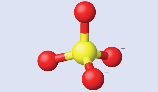
Ammonium sulfate is important as a fertilizer. What is the hybridization of the sulfur atom in the sulfate ion, [latex]{\text{SO}}_{4}^{2-}[/latex]?
The Lewis structure of sulfate shows there are four regions of electron density. The hybridization is sp 3 .

Check Your Learning

Example 2: Assigning Hybridization
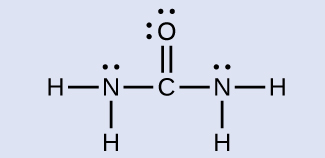
Urea, NH 2 C(O)NH 2 , is sometimes used as a source of nitrogen in fertilizers. What is the hybridization of each nitrogen and carbon atom in urea?
The Lewis structure of urea is

The nitrogen atoms are surrounded by four regions of electron density, which arrange themselves in a tetrahedral electron-pair geometry. The hybridization in a tetrahedral arrangement is sp 3 (Figure 8.21). This is the hybridization of the nitrogen atoms in urea. The carbon atom is surrounded by three regions of electron density, positioned in a trigonal planar arrangement. The hybridization in a trigonal planar electron pair geometry is sp 2 (Figure 8.21), which is the hybridization of the carbon atom in urea.
Acetic acid, H 3 CC(O)OH, is the molecule that gives vinegar its odor and sour taste. What is the hybridization of the two carbon atoms in acetic acid?

Key Concepts and Summary
We can use hybrid orbitals, which are mathematical combinations of some or all of the valence atomic orbitals, to describe the electron density around covalently bonded atoms. These hybrid orbitals either form sigma (σ) bonds directed toward other atoms of the molecule or contain lone pairs of electrons. We can determine the type of hybridization around a central atom from the geometry of the regions of electron density about it. Two such regions imply sp hybridization; three, sp 2 hybridization; four, sp 3 hybridization; five, sp 3 d hybridization; and six, sp 3 d 2 hybridization. Pi (π) bonds are formed from unhybridized atomic orbitals ( p or d orbitals).
- Why is the concept of hybridization required in valence bond theory?
- Explain why a carbon atom cannot form five bonds using sp 3 d hybrid orbitals.
- [latex]{\text{PO}}_{4}^{\text{3-}}[/latex]
- A molecule with the formula AB 3 could have one of four different shapes. Give the shape and the hybridization of the central A atom for each.

- circular S 8 molecule
- SO 2 molecule
- SO 3 molecule
- H 2 SO 4 molecule (the hydrogen atoms are bonded to oxygen atoms)
- Draw a Lewis structure.
- Predict the geometry about the carbon atom.
- Determine the hybridization of each type of carbon atom.
- What is the formula of the compound?
- Write a Lewis structure for the compound.
- Predict the shape of the molecules of the compound.
- What hybridization is consistent with the shape you predicted?
- Write a Lewis structure.
- What are the electron pair and molecular geometries of the internal oxygen and nitrogen atoms in the HNO 2 molecule?
- What is the hybridization on the internal oxygen and nitrogen atoms in HNO 2 ?

- Write Lewis structures for P 4 S 3 and the [latex]{\text{ClO}}_{3}^{-}[/latex] ion.
- Describe the geometry about the P atoms, the S atom, and the Cl atom in these species.
- Assign a hybridization to the P atoms, the S atom, and the Cl atom in these species.
- Determine the oxidation states and formal charge of the atoms in P 4 S 3 and the [latex]{\text{ClO}}_{3}^{-}[/latex] ion.

- Write Lewis structures for NF 3 and PF 5 . On the basis of hybrid orbitals, explain the fact that NF 3 , PF 3 , and PF 5 are stable molecules, but NF 5 does not exist.
- In addition to NF 3 , two other fluoro derivatives of nitrogen are known: N 2 F 4 and N 2 F 2 . What shapes do you predict for these two molecules? What is the hybridization for the nitrogen in each molecule?
1. Hybridization is introduced to explain the geometry of bonding orbitals in valance bond theory.
3. There are no d orbitals in the valence shell of carbon.
5. trigonal planar, sp 2 , trigonal pyramidal (one lone pair on A) sp 3 , T-shaped (two lone pairs on A sp 3 d , or (three lone pair on A) sp 3 d 2
7. The Lewis structures and predicted molecular geometries are as follows:

9. The answers are as follows:
- [latex]\frac{\text{77.55 g}}{\text{131.29 g}{\text{ mol}}^{-1}}=0.5907\text{ mol}[/latex]
- [latex]\frac{\text{22.45 g}}{\text{18.998 g}{\text{ mol}}^{-1}}=\text{1.182 mol}[/latex]
Find the ratio by dividing by the smaller value.
- [latex]\frac{1.182}{0.5907}=2.001[/latex]

- There are 22 electrons, 16 of which are used in the bond, leaving six electrons in the three pairs of unbonded electrons centered about the Xe. These unshared electrons are in a trigonal planar shape with the bonding pairs above and below the plane. Therefore, XeF 2 is linear.
- sp 3 d hybridization is consistent with the linear shape.
11. The answers are as follows:

- P atoms, trigonal pyramidal; S atoms, bent, with two lone pairs; Cl atoms, trigonal pyramidal;
- Hybridization about P, S, and Cl is, in all cases, sp 3 ;
- Oxidation states P +1, S [latex]-1\frac{1}{3},[/latex] Cl +5, O –2. Formal charges: P 0; S 0; Cl +2: O –1
13. Phosphorus and nitrogen can form sp 3 hybrids to form three bonds and hold one lone pair in PF 3 and NF 3 , respectively. However, nitrogen has no valence d orbitals, so it cannot form a set of sp 3 d hybrid orbitals to bind five fluorine atoms in NF 5 . Phosphorus has d orbitals and can bind five fluorine atoms with sp 3 d hybrid orbitals in PF 5 .

hybrid orbital: orbital created by combining atomic orbitals on a central atom
hybridization: model that describes the changes in the atomic orbitals of an atom when it forms a covalent compound
sp hybrid orbital: one of a set of two orbitals with a linear arrangement that results from combining one s and one p orbital
sp 2 hybrid orbital: one of a set of three orbitals with a trigonal planar arrangement that results from combining one s and two p orbitals
sp 3 hybrid orbital: one of a set of four orbitals with a tetrahedral arrangement that results from combining one s and three p orbitals
sp 3 d hybrid orbital: one of a set of five orbitals with a trigonal bipyramidal arrangement that results from combining one s , three p , and one d orbital
sp 3 d 2 hybrid orbital: one of a set of six orbitals with an octahedral arrangement that results from combining one s , three p , and two d orbitals
- Chemistry. Provided by : OpenStax College. Located at : http://openstaxcollege.org . License : CC BY: Attribution . License Terms : Download for free at https://openstaxcollege.org/textbooks/chemistry/get

Chapter 7: Advanced Theories of Covalent Bonding
7.5 Hybrid Atomic Orbitals
Learning outcomes.
- Explain the concept of atomic orbital hybridization
- Determine the hybrid orbitals associated with various molecular geometries
Thinking in terms of overlapping atomic orbitals is one way for us to explain how chemical bonds form in diatomic molecules. However, to understand how molecules with more than two atoms form stable bonds, we require a more detailed model. As an example, let us consider the water molecule, in which we have one oxygen atom bonding to two hydrogen atoms. Oxygen has the electron configuration 1 s 2 2 s 2 2 p 4 , with two unpaired electrons (one in each of the two 2p orbitals). Valence bond theory would predict that the two [latex]\ce{O-H}[/latex] bonds form from the overlap of these two 2 p orbitals with the 1 s orbitals of the hydrogen atoms. If this were the case, the bond angle would be 90°, as shown in Figure 7.5.1 ( note that orbitals may sometimes be drawn in an elongated “balloon” shape rather than in a more realistic “plump” shape in order to make the geometry easier to visualize ), because p orbitals are perpendicular to each other.. Experimental evidence shows that the bond angle is 104.5°, not 90°. The prediction of the valence bond theory model does not match the real-world observations of a water molecule; a different model is needed.
Quantum-mechanical calculations suggest why the observed bond angles in [latex]\ce{H2O}[/latex] differ from those predicted by the overlap of the 1 s orbital of the hydrogen atoms with the 2 p orbitals of the oxygen atom. The mathematical expression known as the wave function, ψ , contains information about each orbital and the wavelike properties of electrons in an isolated atom. When atoms are bound together in a molecule, the wave functions combine to produce new mathematical descriptions that have different shapes. This process of combining the wave functions for atomic orbitals is called hybridization and is mathematically accomplished by the linear combination of atomic orbitals , LCAO, (a technique that we will encounter again later). The new orbitals that result are called hybrid orbital . The valence orbitals in an isolated oxygen atom are a 2 s orbital and three 2 p orbitals. The valence orbitals in an oxygen atom in a water molecule differ; they consist of four equivalent hybrid orbitals that point approximately toward the corners of a tetrahedron ( Figure 7.5.2 ). Consequently, the overlap of the [latex]\ce{O}[/latex] and [latex]\ce{H}[/latex] orbitals should result in a tetrahedral bond angle (109.5°). The observed angle of 104.5° is experimental evidence for which quantum-mechanical calculations give a useful explanation: Valence bond theory must include a hybridization component to give accurate predictions.
The following ideas are important in understanding hybridization:
- Hybrid orbitals do not exist in isolated atoms. They are formed only in covalently bonded atoms.
- Hybrid orbitals have shapes and orientations that are very different from those of the atomic orbitals in isolated atoms.
- A set of hybrid orbitals is generated by combining atomic orbitals. The number of hybrid orbitals in a set is equal to the number of atomic orbitals that were combined to produce the set.
- All orbitals in a set of hybrid orbitals are equivalent in shape and energy.
- The type of hybrid orbitals formed in a bonded atom depends on its electron-pair geometry as predicted by the VSEPR theory.
- Hybrid orbitals overlap to form σ bonds. Unhybridized orbitals overlap to form π bonds.
In the following sections, we shall discuss the common types of hybrid orbitals.
sp Hybridization
The beryllium atom in a gaseous [latex]\ce{BeCl2}[/latex] molecule is an example of a central atom with no lone pairs of electrons in a linear arrangement of three atoms. There are two regions of valence electron density in the [latex]\ce{BeCl2}[/latex] molecule that correspond to the two covalent [latex]\ce{Be-Cl}[/latex] bonds. To accommodate these two electron domains, two of the Be atom’s four valence orbitals will mix to yield two hybrid orbitals. This hybridization process involves mixing of the valence s orbital with one of the valence p orbitals to yield two equivalent sp hybrid orbital that are oriented in a linear geometry ( Figure 7.5.3 ). In this figure, the set of sp orbitals appears similar in shape to the original p orbital, but there is an important difference. The number of atomic orbitals combined always equals the number of hybrid orbitals formed. The p orbital is one orbital that can hold up to two electrons. The sp set is two equivalent orbitals that point 180° from each other. The two electrons that were originally in the s orbital are now distributed to the two sp orbitals, which are half filled. In gaseous [latex]\ce{BeCl2}[/latex], these half-filled hybrid orbitals will overlap with orbitals from the chlorine atoms to form two identical [latex]\sigma[/latex] bonds.
We illustrate the electronic differences in an isolated Be atom and in the bonded Be atom in the orbital energy-level diagram in Figure 7.5.4 . These diagrams represent each orbital by a horizontal line (indicating its energy) and each electron by an arrow. Energy increases toward the top of the diagram. We use one upward arrow to indicate one electron in an orbital and two arrows (up and down) to indicate two electrons of opposite spin.
Any central atom surrounded by just two regions of valence electron density in a molecule will exhibit sp hybridization. Other examples include the mercury atom in the linear [latex]\ce{HgCl2}[/latex] molecule, the zinc atom in [latex]\ce{Zn(CH3)2}[/latex], which contains a linear [latex]\ce{C-Zn-C}[/latex] arrangement, and the carbon atoms in [latex]\ce{HCCH}[/latex] and [latex]\ce{CO2}[/latex].
sp 2 Hybridization
The valence orbitals of a central atom surrounded by three regions of electron density consist of a set of three sp 2 hybrid orbital and one unhybridized p orbital. This arrangement results from sp 2 hybridization, the mixing of one s orbital and two p orbitals to produce three identical hybrid orbitals oriented in a trigonal planar geometry ( Figure 7.5.5 ).
Although quantum mechanics yields the “plump” orbital lobes as depicted in Figure 7.5.5 , sometimes for clarity these orbitals are drawn thinner and without the minor lobes, as in Figure 7.5.6 , to avoid obscuring other features of a given illustration.
We will use these “thinner” representations whenever the true view is too crowded to easily visualize.
The observed structure of the borane molecule, [latex]\ce{BH3}[/latex], suggests sp 2 hybridization for boron in this compound. The molecule is trigonal planar, and the boron atom is involved in three bonds to hydrogen atoms ( Figure 7.5.7 ).
We can illustrate the comparison of orbitals and electron distribution in an isolated boron atom and in the bonded atom in [latex]\ce{BH3}[/latex] as shown in the orbital energy level diagram in Figure 7.5.8 . We redistribute the three valence electrons of the boron atom in the three sp 2 hybrid orbitals, and each boron electron pairs with a hydrogen electron when [latex]\ce{B-H}[/latex] bonds form.
sp 3 Hybridization
The valence orbitals of an atom surrounded by a tetrahedral arrangement of bonding pairs and lone pairs consist of a set of four sp 3 hybrid orbital . The hybrids result from the mixing of one s orbital and all three p orbitals that produces four identical sp 3 hybrid orbitals ( Figure 7.5.10 ). Each of these hybrid orbitals points toward a different corner of a tetrahedron.
A molecule of methane, [latex]\ce{CH4}[/latex], consists of a carbon atom surrounded by four hydrogen atoms at the corners of a tetrahedron. The carbon atom in methane exhibits sp 3 hybridization. We illustrate the orbitals and electron distribution in an isolated carbon atom and in the bonded atom in [latex]\ce{CH4}[/latex] in Figure 7.5.11 . The four valence electrons of the carbon atom are distributed equally in the hybrid orbitals, and each carbon electron pairs with a hydrogen electron when the [latex]\ce{C-H}[/latex] bonds form.
In a methane molecule, the 1 s orbital of each of the four hydrogen atoms overlaps with one of the four sp 3 orbitals of the carbon atom to form a sigma ([latex]\sigma[/latex]) bond. This results in the formation of four strong, equivalent covalent bonds between the carbon atom and each of the hydrogen atoms to produce the methane molecule, [latex]\ce{CH4}[/latex].
The structure of ethane, [latex]\ce{C2H6}[/latex] , is similar to that of methane in that each carbon in ethane has four neighboring atoms arranged at the corners of a tetrahedron—three hydrogen atoms and one carbon atom ( Figure 7.5.12 ). However, in ethane an sp 3 orbital of one carbon atom overlaps end to end with an sp 3 orbital of a second carbon atom to form a σ bond between the two carbon atoms. Each of the remaining sp 3 hybrid orbitals overlaps with an s orbital of a hydrogen atom to form carbon–hydrogen σ bonds. The structure and overall outline of the bonding orbitals of ethane are shown in Figure 7.5.12 . The orientation of the two [latex]\ce{CH3}[/latex] groups is not fixed relative to each other. Experimental evidence shows that rotation around [latex]\sigma[/latex] bonds occurs easily.
An sp 3 hybrid orbital can also hold a lone pair of electrons. For example, the nitrogen atom in ammonia is surrounded by three bonding pairs and a lone pair of electrons directed to the four corners of a tetrahedron. The nitrogen atom is sp 3 hybridized with one hybrid orbital occupied by the lone pair. The molecular structure of water is consistent with a tetrahedral arrangement of two lone pairs and two bonding pairs of electrons. Thus we say that the oxygen atom is sp 3 hybridized, with two of the hybrid orbitals occupied by lone pairs and two by bonding pairs. Since lone pairs occupy more space than bonding pairs, structures that contain lone pairs have bond angles slightly distorted from the ideal. Perfect tetrahedra have angles of 109.5°, but the observed angles in ammonia (107.3°) and water (104.5°) are slightly smaller. Other examples of sp 3 hybridization include [latex]\ce{CCl4}[/latex], [latex]\ce{PCl3}[/latex], and [latex]\ce{NCl3}[/latex].
sp 3 d and sp 3 d 2 Hybridization
To describe the five bonding orbitals in a trigonal bipyramidal arrangement, we must use five of the valence shell atomic orbitals (the s orbital, the three p orbitals, and one of the d orbitals), which gives five sp 3 d hybrid orbital . With an octahedral arrangement of six hybrid orbitals, we must use six valence shell atomic orbitals (the s orbital, the three p orbitals, and two of the d orbitals in its valence shell), which gives six sp 3 d 2 hybrid orbital . These hybridizations are only possible for atoms that have d orbitals in their valence subshells (that is, not those in the first or second period).
In a molecule of phosphorus pentachloride, [latex]\ce{PCl5}[/latex], there are five [latex]\ce{P-Cl}[/latex] bonds (thus five pairs of valence electrons around the phosphorus atom) directed toward the corners of a trigonal bipyramid. We use the 3 s orbital, the three 3 p orbitals, and one of the 3 d orbitals to form the set of five sp 3 d hybrid orbitals ( Figure 7.5.14 ) that are involved in the P–Cl bonds. Other atoms that exhibit sp 3 d hybridization include the sulfur atom in [latex]\ce{SF4}[/latex] and the chlorine atoms in [latex]\ce{ClF3}[/latex] and in [latex]\ce{ClF4+}[/latex]. (The electrons on fluorine atoms are omitted for clarity.)
The sulfur atom in sulfur hexafluoride, [latex]\ce{SF6}[/latex], exhibits sp 3 d 2 hybridization. A molecule of sulfur hexafluoride has six bonding pairs of electrons connecting six fluorine atoms to a single sulfur atom ( Figure 7.5.15 ). There are no lone pairs of electrons on the central atom. To bond six fluorine atoms, the 3 s orbital, the three 3 p orbitals, and two of the 3 d orbitals form six equivalent sp 3 d 2 hybrid orbitals, each directed toward a different corner of an octahedron. Other atoms that exhibit sp 3 d 2 hybridization include the phosphorus atom in [latex]{\ce{PCl}}_{6}^{-},[/latex] the iodine atom in the interhalogens [latex]{\ce{IF}}_{6}^{\text{+}}[/latex], [latex]\ce{IF}_{5}[/latex], [latex]{\ce{ICl}}_{4}^{-}[/latex], [latex]{\ce{IF}}_{4}^{-}[/latex] and the xenon atom in [latex]\ce{XeF}_{4}[/latex].
Assignment of Hybrid Orbitals to Central Atoms
The hybridization of an atom is determined based on the number of regions of electron density that surround it. The geometrical arrangements characteristic of the various sets of hybrid orbitals are shown in Figure 7.5.16 . These arrangements are identical to those of the electron-pair geometries predicted by VSEPR theory. VSEPR theory predicts the shapes of molecules, and hybrid orbital theory provides an explanation for how those shapes are formed. To find the hybridization of a central atom, we can use the following guidelines:
- Determine the Lewis structure of the molecule.
- Determine the number of regions of electron density around an atom using VSEPR theory, in which single bonds, multiple bonds, radicals, and lone pairs each count as one region.
- Assign the set of hybridized orbitals from Figure 7.5.16 that corresponds to this geometry.
It is important to remember that hybridization was devised to rationalize experimentally observed molecular geometries. The model works well for molecules containing small central atoms, in which the valence electron pairs are close together in space. However, for larger central atoms, the valence-shell electron pairs are farther from the nucleus, and there are fewer repulsions. Their compounds exhibit structures that are often not consistent with VSEPR theory, and hybridized orbitals are not necessary to explain the observed data. For example, we have discussed the [latex]\ce{H-O-H}[/latex] bond angle in [latex]\ce{H2O}[/latex], 104.5°, which is more consistent with sp 3 hybrid orbitals (109.5°) on the central atom than with 2 p orbitals (90°). Sulfur is in the same group as oxygen, and H 2 S has a similar Lewis structure. However, it has a much smaller bond angle (92.1°), which indicates much less hybridization on sulfur than oxygen. Continuing down the group, tellurium is even larger than sulfur, and for [latex]\ce{H2Te}[/latex], the observed bond angle (90°) is consistent with overlap of the 5 p orbitals, without invoking hybridization. We invoke hybridization where it is necessary to explain the observed structures.
Example 7.5.1: Assigning Hybridization
Ammonium sulfate is important as a fertilizer. What is the hybridization of the sulfur atom in the sulfate ion, [latex]\ce{SO4^{2-}}[/latex]?
The Lewis structure of sulfate shows there are four regions of electron density. The hybridization is sp 3 .
Check Your Learning
Example 7.5.2: assigning hybridization.
Urea, [latex]\ce{NH2C(O)NH2}[/latex], is sometimes used as a source of nitrogen in fertilizers. What is the hybridization of each nitrogen and carbon atom in urea?
The Lewis structure of urea is
The nitrogen atoms are surrounded by four regions of electron density, which arrange themselves in a tetrahedral electron-pair geometry. The hybridization in a tetrahedral arrangement is sp 3 . This is the hybridization of the nitrogen atoms in urea. The carbon atom is surrounded by three regions of electron density, positioned in a trigonal planar arrangement. The hybridization in a trigonal planar electron pair geometry is sp 2 , which is the hybridization of the carbon atom in urea.
Key Concepts and Summary
We can use hybrid orbitals, which are mathematical combinations of some or all of the valence atomic orbitals, to describe the electron density around covalently bonded atoms. These hybrid orbitals either form sigma ([latex]\sigma[/latex]) bonds directed toward other atoms of the molecule or contain lone pairs of electrons. We can determine the type of hybridization around a central atom from the geometry of the regions of electron density about it. Two such regions imply sp hybridization; three, sp 2 hybridization; four, sp 3 hybridization; five, sp 3 d hybridization; and six, sp 3 d 2 hybridization. Pi (π) bonds are formed from unhybridized atomic orbitals ( p or d orbitals).
- [latex]\ce{BeH2}[/latex]
- [latex]\ce{SF6}[/latex]
- [latex]\ce{PO4^{3-}}[/latex]
- [latex]\ce{PCl5}[/latex]
- A molecule with the formula AB 3 could have one of four different shapes. Give the shape and the hybridization of the central A atom for each.
- Write Lewis structures for [latex]\ce{NF3}[/latex] and [latex]\ce{PF5}[/latex]. On the basis of hybrid orbitals, explain the fact that [latex]\ce{NF3}[/latex], [latex]\ce{PF3}[/latex], and [latex]\ce{PF5}[/latex] are stable molecules, but [latex]\ce{NF5}[/latex] does not exist.
2. trigonal planar, sp 2 , trigonal pyramidal (one lone pair on A) sp 3 , T-shaped (two lone pairs on A sp 3 d , or (three lone pair on A) sp 3 d 2
3. Phosphorus and nitrogen can form sp 3 hybrids to form three bonds and hold one lone pair in [latex]\ce{PF3}[/latex] and [latex]\ce{NF3}[/latex], respectively. However, nitrogen has no valence d orbitals, so it cannot form a set of sp 3 d hybrid orbitals to bind five fluorine atoms in [latex]\ce{NF5}[/latex]. Phosphorus has d orbitals and can bind five fluorine atoms with sp 3 d hybrid orbitals in [latex]\ce{PF5}[/latex].
hybrid orbital: orbital created by combining atomic orbitals on a central atom
hybridization: model that describes the changes in the atomic orbitals of an atom when it forms a covalent compound
sp hybrid orbital: one of a set of two orbitals with a linear arrangement that results from combining one s and one p orbital
sp 2 hybrid orbital: one of a set of three orbitals with a trigonal planar arrangement that results from combining one s and two p orbitals
sp 3 hybrid orbital: one of a set of four orbitals with a tetrahedral arrangement that results from combining one s and three p orbitals
sp 3 d hybrid orbital: one of a set of five orbitals with a trigonal bipyramidal arrangement that results from combining one s , three p , and one d orbital
sp 3 d 2 hybrid orbital: one of a set of six orbitals with an octahedral arrangement that results from combining one s , three p , and two d orbitals
CC licensed content, Shared previously
- Chemistry 2e. Provided by : OpenStax. Located at : https://openstax.org/ . License : CC BY: Attribution . License Terms : Access for free at https://openstax.org/books/chemistry-2e/pages/1-introduction
one of a set of two orbitals with a linear arrangement that results from combining one s and one p orbital
orbital created by combining atomic orbitals on a central atom
one of a set of three orbitals with a trigonal planar arrangement that results from combining one s and two p orbitals
one of a set of four orbitals with a tetrahedral arrangement that results from combining one s and three p orbitals
one of a set of five orbitals with a trigonal bipyramidal arrangement that results from combining one s, three p, and one d orbital
one of a set of six orbitals with an octahedral arrangement that results from combining one s, three p, and two d orbitals
Chemistry Fundamentals Copyright © by Dr. Julie Donnelly, Dr. Nicole Lapeyrouse, and Dr. Matthew Rex is licensed under a Creative Commons Attribution-NonCommercial-ShareAlike 4.0 International License , except where otherwise noted.
Share This Book
- Hybrid Atomic Orbitals
Assignment of Hybrid Orbitals to Central Atoms
The hybridization of an atom is determined based on the number of regions of electron density that surround it. The geometrical arrangements characteristic of the various sets of hybrid orbitals are shown in the table below. These arrangements are identical to those of the electron-pair geometries predicted by VSEPR theory. VSEPR theory predicts the shapes of molecules, and hybrid orbital theory provides an explanation for how those shapes are formed. To find the hybridization of a central atom, we can use the following guidelines:
- Determine the Lewis structure of the molecule.
- Determine the number of regions of electron density around an atom using VSEPR theory, in which single bonds, multiple bonds, radicals, and lone pairs each count as one region.
- Assign the set of hybridized orbitals from the table below that corresponds to this geometry.
It is important to remember that hybridization was devised to rationalize experimentally observed molecular geometries. The model works well for molecules containing small central atoms, in which the valence electron pairs are close together in space. However, for larger central atoms, the valence-shell electron pairs are farther from the nucleus, and there are fewer repulsions. Their compounds exhibit structures that are often not consistent with VSEPR theory, and hybridized orbitals are not necessary to explain the observed data. For example, we have discussed the H–O–H bond angle in H 2 O, 104.5°, which is more consistent with sp 3 hybrid orbitals (109.5°) on the central atom than with 2 p orbitals (90°). Sulfur is in the same group as oxygen, and H 2 S has a similar Lewis structure. However, it has a much smaller bond angle (92.1°), which indicates much less hybridization on sulfur than oxygen. Continuing down the group, tellurium is even larger than sulfur, and for H 2 Te, the observed bond angle (90°) is consistent with overlap of the 5 p orbitals, without invoking hybridization. We invoke hybridization where it is necessary to explain the observed structures.
Assigning Hybridization Ammonium sulfate is important as a fertilizer. What is the hybridization of the sulfur atom in the sulfate ion, $SO_4^{2−}$?
Solution The Lewis structure of sulfate shows there are four regions of electron density. The hybridization is sp 3 .
Check Your Learning What is the hybridization of the selenium atom in SeF 4 ?
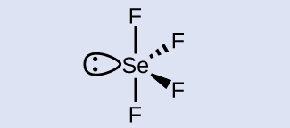
Answer: The selenium atom is sp 3 d hybridized.
Assigning Hybridization Urea, NH 2 C(O)NH 2 , is sometimes used as a source of nitrogen in fertilizers. What is the hybridization of the carbon atom in urea?
Solution The Lewis structure of urea is:
The carbon atom is surrounded by three regions of electron density, positioned in a trigonal planar arrangement. The hybridization in a trigonal planar electron pair geometry is sp 2 ( [link] ), which is the hybridization of the carbon atom in urea.
Check Your Learning Acetic acid, H 3 CC(O)OH, is the molecule that gives vinegar its odor and sour taste.
- Privacy Policy
Read Chemistry
Hybridization: definition, types, rules, examples.
Read Chemistry May 5, 2019 Organic Chemistry , Physical Chemistry
– In this subject, we will discuss the Hybridization: Definition, Types, Rules, and Examples

– While the formation of simple molecules could be explained adequately by the overlap of atomic orbitals , the formation of molecules of Be, B, and C present problems of greater magnitude having no solution with the previous theory.
– To explain fully the tendency of these atoms to form bonds and the shape or geometry of their molecules, a new concept called Hybridization is introduced.
Atomic orbitals and Hybrid orbitals
– According to this concept, we may mix any number of atomic orbitals of an atom, which differ in energy only slightly, to form new orbitals called Hybrid orbitals.
– The mixing orbitals generally belong to the same energy level (say 2s and 2p orbitals may hybridize).
– The total number of hybrid orbitals formed after mixing is invariably equal to the number of atomic orbitals mixed or hybridized.
- An important characteristic of hybrid orbitals is that:
(1) they are all identical in respect of energy and directional character.
(2) They, however, differ from the original atomic orbitals in these respects.
(3) They may also differ from one another in respect of their arrangement in space. i.e., orientation.
(4) Like pure atomic orbitals, the hybrid orbitals of an atom shall have a maximum of two electrons with opposite spin.
(5) Hybrid orbitals of an atom may overlap with other bonding orbitals (pure atomic or hybrid) on other atoms or form molecular orbitals and hence new bonds.
Definition of Hybridization
- Hybridization is defined as the phenomenon of mixing up (or merging) of orbitals of an atom of nearly equal energy, giving rise to entirely new orbitals equal in number to the mixing orbitals and having the same energy contents and identical shapes.
Rules of Hybridization
– For hybridization to occur, it is necessary for the atom to satisfy the following conditions :
(1) Orbitals on a single atom only would undergo hybridization.
(2) There should be very little difference in energy level between the orbitals mixing to form hybrid orbitals.
(3) The number of hybrid orbitals generated is equal to the number of hybridizing orbitals.
(4) The hybrid orbitals assume the direction of the dominating orbitals.
– For example, if s and p orbitals are to hybridize, the s orbital having no directional character, does not contribute towards the direction when p orbitals determine the directional character of the hybrid orbitals.
(5) It is the orbitals that undergo hybridization and not the electrons.
– For example, four orbitals of an oxygen atom (2 2, 2 2, 2 1, 2 1 ) s px py pz belonging to the second level (i.e., 2s, 2p x , 2p y , 2p z ) can hybridize to give four hybrid orbitals, two of which have two electrons each (as before) and the other two have one electron each.
(6) The electron waves in hybrid orbitals repel each other and thus tend to be farthest apart.
Types of Hybridization
– Since hybridization lends an entirely new shape and orientation to the valence orbitals of an atom, it holds significant importance in determining the shape and geometry of the molecules formed from such orbitals.
– Depending upon the number and nature of the orbitals undergoing by hybridisation, we have various types of hybrid orbitals.
– For instance s, p, and d orbitals of simple atoms may hybridize in the following manner:
sp Hybridization
Sp 2 hybridization, sp 3 hybridization, hybridization involving (d) orbitals.
– The mixing of an (s) and a (p) orbital only leads to two hybrid orbitals known as sp hybrid orbitals after the name of an s and a p orbital involved in the process of hybridisation. The process is called sp hybridization .
– In sp hybridization process, Each sp orbital has 50%, s-character, and 50% p-character.
– Orbitals thus generated are the seat of electrons which have a tendency to repel and be farther apart.
– To do so the new orbitals arrange themselves along a line and are, therefore, often referred to as Linear hybrid orbitals.
– This gives an angle of 180º between the axes of the two orbitals.
– The following Figure that an sp orbital has two lobes (a character of p orbital) one of which is farther than the corresponding s or p orbitals and also protrudes farther along the axis.
– It is this bigger lobe that involves itself in the process of an overlap with orbitals of other atoms to form bonds.
– It will be seen later on that the smaller lobes of hybrid orbitals are neglected while considering bond formation.

– Examples of sp Hybridization : BeF 2 , BeCl 2 , etc.
– When an s and two p orbitals mix up to hybridize, there result three new orbitals called sp 2 hybrid orbitals (spoken as ‘sp two’).
– In the sp 2 hybridization process, Each sp 2 hybrid orbital has 33% s-character and 67% p-character.
– As the three orbitals undergoing hybridisation lie in a plane, so do the new orbitals.
– They have to lie farthest apart in a plane which can happen if they are directed at an angle of 120º to one another as shown in Fig. (b).
– It is for this reason that sp 2 hybrid orbitals are also called Trigonal hybrids, the process being referred to as Trigonal hybridization.
– The sp 2 hybrid orbitals resemble in shape with that of sp hybrid orbitals but are slightly fatter.

– Examples of sp 2 Hybridization: BF 3 , NO 3 – , etc.
– The four new orbitals formed by mixing an s and three p orbitals of an atom are known as sp 3 hybrid orbitals .
– In sp 3 hybridization process, Each sp 3 hybrid orbital has 25% s-character and 75% p-character.
– Since the mixing of orbitals takes place in space, the four hybrid orbital would also lie in space.
– An arrangement in space that keeps them farthest apart is that of a tetrahedron. Thus each of the four hybrid orbitals is directed towards the four corners of a regular tetrahedron as shown in Fig (b).
– Because of their tetrahedral disposition, this type of hybridization is also called Tetrahedral hybridisation.
– They are of the same shape as that of the previous two types but bigger in size.
– They are disposed in a manner such that the angle between them is 109.5º as shown in the following Figure:

– Examples of sp 3 Hybridization: CH 4 , SO 4 2- , ClO 4 – , etc.
– There are several types of hybridization involving d orbitals.
– Since the d orbitals have a relatively complex shape, we will consider here only some of the common types.
– The most important of these are sp 3 d hybridization, sp 3 d 2 hybridization and sp 2 d hybridization.
– In sp 3 d hybridization, the orbitals involved are one of s type, three of p type, and one of d type.
– The five new orbitals will be farthest apart by arranging three of them in a plane at an angle of 120º to one another and the other two in a direction perpendicular to the plane.
– The figure obtained by joining the ends assumes the shape of a trigonal bipyramid.
– This type of hybridization is, therefore, called Trigonal bipyramidal hybridization.
– When two (d) type of orbitals take part in hybridisation with one s type and three p type orbitals, six hybrid orbitals called sp 3 d 2 hybrid orbitals are created.
– To be away from one another four of them are dispersed in a plane at an angle of 90º each and the rest two are directed up and below this plane in a direction perpendicular to it.
– On joining their corners, an octahedron results and this type of hybridisation also gets the name Octahedral hybridization
– So far we have been considering the hybridisation of orbitals belonging to the same energy level (say 3s, 3p, and 3d orbitals) of an atom. But this may not necessarily be so always.
– In fact, there is very little energy difference between 3d, 4s, and 4p orbitals which may undergo sp 2 d hybridization.
– The d orbital involved in this type of hybridization has the same planar character as the two p orbitals have and the hybrid orbitals will also be planar, dispersed in such a way so as to be farthest apart i.e., subtending an angle of 90º between them.
– This gives a square planar arrangement for them and the hybridization is, therefore, called Square planar hybridization.
– The directional characters of the types of hybridization discussed above are summarised in the following Figure:

Related Articles

Carnot Cycle – Definition, Theorem, Efficiency, Derivation
May 22, 2024

Synthesis of Ethers

Entropy : Definition, Units, Solved Problems
May 21, 2024
Williamson Ether Synthesis : Mechanism, Examples

Macromolecules : Definition and Molecular Weight
May 20, 2024

Spectroscopy of Ethers : IR, Mass, 13C NMR, 1H NMR
One comment.

The are elaborate and informative 👌
Leave a Reply Cancel reply
Your email address will not be published. Required fields are marked *
Save my name, email, and website in this browser for the next time I comment.
Browse Course Material
Course info.
- Prof. Donald Sadoway
Departments
- Materials Science and Engineering
As Taught In
- Chemical Engineering
Learning Resource Types
Introduction to solid state chemistry, 10. hybridized & molecular orbitals; paramagnetism.
« Previous | Next »
Session Overview
| Bonding and Molecules | |
| linear combination of atomic orbitals–molecular orbitals (LCAO-MO): energy level diagrams, bonding and anti-bonding orbitals, and hybridization, paramagnetism and diamagnetism | |
| Wolfgang Pauli, primary bond, ionic bond, covalent bond, metallic bond, electronegativity, metal, non-metal, superposition, alkali metal, node, lobe, nodal plane, electron density, alloy, electronic conductivity, ionic conductivity, molten salt, liquid metal, energy level diagram, atomic orbital, molecular orbital, bonding orbital, antibonding orbital, paramagnetism, sigma bond, pi bond, hybridization, single bond, double bond, triple bond, diamagnetism, octet stability, polar bond, polar molecule, nonpolar molecule, homonuclear molecule, heteronuclear molecule, Schrödinger’s equation, linear superposition, atomic orbital wavefunction, conservation of orbital states, Aufbau principle, quantum numbers, Pauli exclusion principle, Hund’s rule, bonding electron, nonbonding electron, unpaired electrons, Lewis structure, electron transfer | |
| ethylene (C H ), methane (CH ), carbon (C), acetylene (C H ), titanium tetrachloride (TiCl ), sulfur hexafluoride (SF ), bromine pentafluoride (BrF ), iodine tetrafluoride (IF ), helium (He), dilithium (Li ), disodium (Na ), nitrogen (N ), oxygen (O ), fluorine (F ) | |
| sodium vapor lamps |
Prerequisites
Before starting this session, you should be familiar with:
- Session 9: Drawing Lewis Structures
Looking Ahead
Prof. Sadoway discusses the shapes of molecules ( Session 11 ).
Learning Objectives
After completing this session, you should be able to:
- Define polar bond , polar molecule , dipole moment.
- Identify three types of primary bonds : ionic, covalent, metallic.
- Explain why homonuclear molecules and molecules containing symmetric arrangements of identical polar bonds must be nonpolar .
- Sketch energy level diagrams for molecules using LCAO-MO, and identify the bonding orbitals and antibonding orbitals.
- Explain how paramagnetism occurs**.**
- Describe the components of sigma bonds and pi bonds.
- Explain the source of electronic conductivity and ionic conductivity.
Archived Lecture Notes #2 (PDF) , Section 3
| Book Chapters | Topics |
|---|---|
| 9.2, “Localized Bonding and Hybrid Atomic Orbitals.” | Valence bond theory: a localized bonding approach; hybridization of and orbitals; hybridization using orbitals |
| 9.3, “Delocalized Bonding and Molecular Orbitals.” | Molecular orbital theory: a delocalized bonding approach; bond order in molecular orbital theory; molecular orbitals formed from and atomic orbitals; molecular orbital diagrams for second-period homonuclear diatomic molecules; molecular orbitals in heteronuclear diatomic molecules |
| 9.4, “Combining the Valence Bond and Molecular Orbital Approaches.” | Multiple bonds; molecular orbitals and resonance structures |
Lecture Video
- Download video
- Download transcript
Lecture Slides (PDF - 2.1MB)
Lecture Summary
Prof. Sadoway discusses the following concepts:
- Orbitals split into bonding orbitals (lower) and antibonding orbitals (higher). Electrons fill from lowest energy up.
- sigma = no nodal plane separates nuclei
- pi = a nodal plane separates nuclei
- e.g. liquid oxygen is paramagnetic – can be held by a magnetic field
Problems (PDF)
Solutions (PDF)
Textbook Problems
| [Saylor] Sections | Conceptual | Numerical |
|---|---|---|
| 9.2, “Localized Bonding and Hybrid Atomic Orbitals.” | none | 1, 2, 7, 8 |
| 9.3, “Delocalized Bonding and Molecular Orbitals.” | none | 1, 2, 6, 7, 11, 13, 14, 18 |
For Further Study
Wolfgang Pauli - 1945 Nobel Prize in Physics
Other OCW and OER Content
| Content | Provider | Level | Notes |
|---|---|---|---|
| MIT OpenCourseWare | Undergraduate (first-year) |
|

You are leaving MIT OpenCourseWare
- Chemistry Class 11 Notes
- Physical Chemistry
- Organic Chemistry
- Inorganic Chemistry
- Analytical Chemistry
- Biochemistry
- Chemical Elements
- Chemical Compounds
- Chemical Formula
- Real life Application of Chemistry
- Chemistry Class 8 Notes
- Chemistry Class 9 Notes
- Chemistry Class 10 Notes
- Chemistry Class 12 Notes
Chapter 1 - Some Basic Concepts of Chemistry
- Importance of Chemistry in Everyday Life
- What is Matter ?
- Properties of Matter
- Measurement Uncertainty
- Laws of Chemical Combination
- Dalton's Atomic Theory
- Gram Atomic and Gram Molecular Mass
- Mole Concept
- Percentage Composition - Definition, Formula, Examples
- Stoichiometry and Stoichiometric Calculations
Chapter 2 - Structure of Atom
- Composition of an Atom
- Atomic Structure
- Developments Leading to Bohr's Model of Atom
- Bohr's Model of the Hydrogen Atom
- Quantum Mechanical Atomic Model
Chapter 3 - Classification of Elements and Periodicity in Properties
- Classification of Elements
- Periodic Classification of Elements
- Modern Periodic Law
- 118 Elements and Their Symbols
- Electronic Configuration in Periods and Groups
- Electron Configuration
- S Block Elements
- Periodic Table Trends
Chapter 4 - Chemical Bonding and Molecular Structure
- Chemical Bonding
- Bond Parameters - Definition, Order, Angle, Length
- VSEPR Theory
- Valence Bond Theory
Hybridization
- Molecular Orbital Theory
- Hydrogen Bonding
Chapter 5 - Thermodynamics
- Basics Concepts of Thermodynamics
- Applications of First Law of Thermodynamics
- Internal Energy as a State of System
- Enthalpy Change of a Reaction
- Enthalpies for Different Types of Reactions
- What is Spontaneity? - Definition, Types, Gibbs Energy
- Gibbs Energy Change and Equilibrium
Chapter 6 - Equilibrium
- Equilibrium in Physical Processes
- Equilibrium in Chemical Processes
- Law of Chemical Equilibrium and Equilibrium Constant
- Difference between Homogeneous and Heterogeneous Equilibria
- Applications of Equilibrium Constants
- What is the Relation between Equilibrium Constant, Reaction Quotient and Gibbs Energy?
- Factors Affecting Chemical Equilibrium
- Ionic Equilibrium
- Acids, Bases and Salts
- Ionization of Acids and Bases
- Buffer Solution
- Solubility Equilibria
Chapter 7 - Redox Reactions
- Redox Reactions
- Redox Reactions in terms of Electron Transfer
- Oxidation Number | Definition, How To Find, Examples
- Redox Reactions and Electrode Processes
Chapter 8 - Organic Chemistry – Some Basic Principles and Techniques
- Organic Chemistry - Some Basic Principles and Techniques
- What is Catenation and Tetravalency?
- Structural Representations of Organic Compounds
- Classification of Organic Compounds
- IUPAC Nomenclature of Organic Compounds
- Fundamental Concepts in Organic Reaction Mechanism
- Purification of Organic Compounds
- Qualitative Analysis of Organic Compounds
- What is Quantitative Analysis?
Chapter 9 - Hydrocarbons
- What are Hydrocarbons?
- Classification of Hydrocarbons
- Alkanes - Definition, Nomenclature, Preparation, Properties
- Alkenes - Definition, Nomenclature, Preparation, Properties
- Alkynes - Definition, Structure, Preparation, Properties
- Aromatic Compounds
The concept of hybridization is defined as the process of combining two atomic orbitals to create a new type of hybridized orbitals. This intermixing typically results in the formation of hybrid orbitals with completely different energies, shapes, and so on. Hybridization is primarily carried out by atomic orbitals of the same energy level. However, both fully filled and half-filled orbitals can participate in this process if their energies are equal. The concept of hybridization is an extension of valence bond theory that helps us understand bond formation, bond energies, and bond lengths.
What is Hybridization?
When two atomic orbitals combine to form a hybrid orbital in a molecule, the energy of the orbitals of individual atoms is redistributed to give orbitals of equivalent energy. This is known as hybridization.
The atomic orbitals of comparable energies are mixed together during the hybridization process, which mostly involves the merging of two orbitals or two ‘p’ orbitals or the mixing of an ‘s’ orbital with a ‘p’ orbital as well as an ‘s’ orbital with a ‘d’ orbital.
Hybrid orbitals are the new orbitals formed as a result of this process. More importantly, hybrid orbitals can be used to explain atomic bonding properties and molecular geometry. Carbon , for example, forms four single bonds in which the valence-shell s orbital combines with three valence-shell p orbitals. This combination generates four equivalent sp 3 mixtures. These will be arranged in a tetrahedral pattern around the carbon, which is bonded to four different atoms.
Steps to determine the type of Hybridisation
To understand the type of hybridization in an atom or an ion, the following rules must be followed.
- First, determine the total number of valence electrons contained in an atom or ion.
- Then, count the number of lone pairs attached to that atom or ion.
- Now, the number of orbitals required can be calculated by adding the number of duplex or octet and the number of lone pairs of electrons.
- It should be noted that the geometry of orbitals in atoms or ions is different when there is no lone pair of electrons.
Features of Hybridization
- Hybridization occurs between atomic orbitals with equal energies.
- The number of hybrid orbitals formed equals the number of atomic orbitals that mix.
- It is not required for all half-filled orbitals to participate in hybridization. Even orbitals that are completely filled but have slightly varying energy can participate.
- Hybridization occurs only during bond formation, not in a single gaseous atom.
- If the hybridization of the molecule is known, the molecule’s shape can be predicted.
- The larger lobe of the hybrid orbital is always positive, while the smaller lobe on the opposite side is always negative.
Types of Hybridization
Hybridization can be classified as sp 3 , sp 2 , sp, sp 3 d, sp 3 d 2 , or sp 3 d 3 based on the types of orbitals involved in mixing.
sp Hybridization
It occurs when one s and one p orbital in an atom’s main shell combine to form two new equivalent orbitals. The newly formed orbitals are known as sp hybridized orbitals. It produces linear molecules at a 180° angle. It entails combining one’s orbital and one ‘p’ orbital of equal energy to produce a new hybrid orbital known as an sp hybridized orbital.
- It’s also known as diagonal hybridization.
- Each sp hybridized orbital contains the same amount of s and p characters.
- All beryllium compounds, such as BeF 2 , BeH 2 , and BeCl 2 , are examples.

sp 2 Hybridization
It occurs when one s and two p orbitals of the same atom’s shell combine to form three equivalent orbitals. The newly formed orbitals are known as sp 2 hybrid orbitals. It’s also known as trigonal hybridization. It entails combining one’s orbital with two ‘p’ orbitals of equal energy to create a new hybrid orbital known as sp 2 . A trigonal symmetry mixture of s and p orbitals is kept at 120 degrees. All three hybrid orbitals remain in the same plane and form a 120° angle with one another.
- Each hybrid orbital formed has a 33.33 % and a 66.66 % ‘p’ character.
- The molecules with a triangular planar shape have a central atom that is linked to three other atoms and is sp 2 hybridized. Boron compounds are examples.

sp 3 Hybridization
When one ‘s’ orbital and three ‘p’ orbitals from the same shell of an atom combine to form four new equivalent orbitals, the hybridization is known as tetrahedral hybridization or sp 3 . The newly formed orbitals are known as sp 3 hybrid orbitals. These are pointed at the four corners of a regular tetrahedron and form a 109°28′ angle with one another.
- The sp 3 hybrid orbitals form a 109.28-degree angle.
- Each hybrid orbital has a 25% s character and a 75% p character.
- Ethane and methane are two examples.

sp 3 d Hybridization
The mixing of 1s orbitals, 3p orbitals, and 1d orbitals results in 5 sp3d hybridized orbitals of equal energy. Their geometry is trigonal bipyramidal. The combination of s, p, and d orbitals results in trigonal bipyramidal symmetry. The equatorial orbitals are three hybrid orbitals that are oriented at a 120° angle to each other and lie in the horizontal plane.
- The remaining two orbitals, known as axial orbitals, are in the vertical plane at 90 degrees plane of the equatorial orbitals.
- Hybridization in Phosphorus Pentachloride, for example (PCl 5 ).

sp 3 d 2 Hybridization
When 1s, 3p, and 2d orbitals combine to form 6 identical sp 3 d 2 hybrid orbitals, the hybridization is called sp 3 d 2 Hybridization. These seven orbitals point to the corners of an octahedron. They are inclined at a 90-degree angle to one another.

sp 3 d 3 Hybridization
It has 1s, 3p, and 3d orbitals, which combine to form 7 identical sp 3 d 3 hybrid orbitals. These seven orbitals point to the corners of a pentagonal bipyramidal. e.g. IF 6 .

Shapes of Hybridization
- Linear : The sp hybridization is caused by the interaction of two-electron groups; the orbital angle is 180°.
- Trigonal planar: Three electron groups are involved, resulting in sp 2 hybridization; the orbitals are 120° apart.
- Tetrahedral: Four electron groups are involved, resulting in sp 3 hybridization; the orbital angle is 109.5°.
- Trigonal bipyramidal: Five electron groups are involved, resulting in sp 3 d hybridization; the orbital angles are 90° and 120°.
- Octahedral: Six electron groups are involved, resulting in sp 3 d 2 hybridization; the orbitals are 90° apart.
FAQs on Hybridization
Question 1: Among sp, sp2, and sp3, which hybrid orbital is more electronegative?
The percentage of s character in sp, sp 2 , and sp 3 hybridised carbon is 50%, 33.33%, and 25%, respectively. Because of the spherical shape of the s orbital, it is attracted evenly from all directions by the nucleus. As a result, an s-character hybrid orbital will be closer to the nucleus and thus more electronegative. As a result, the sp hybridised carbon is the most electronegative.
Question 2: What are hybrid orbitals?
Hybrid orbitals are formed by combining standard atomic orbitals and resulting in the formation of new atomic orbitals.
Question 3: What are the five shapes of hybridization?
Linear, trigonal planar, tetrahedral, trigonal bipyramidal, and octahedral are the five basic shapes of hybridization.
Question 4: Why does the amide molecule look like sp 3 hybridized but is sp 2 ?
If the atom is either enclosed by two or more p orbitals or has a lone pair capable of jumping into a p orbital, the general process of hybridization will change. As a result, in the case of an amide molecule, the lone pair enters a p orbital, resulting in three adjacent parallel p orbitals.
Question 5: What is Bent’s rule?
A central atom connected to numerous groups in a molecule will hybridise, causing orbitals with more s character to be directed towards electropositive groups and orbitals with more p character to be directed towards electronegative groups.
Please Login to comment...
Similar reads.
- School Chemistry
- School Learning
- Chemical-Bonding
- Chemistry-Class-11
Improve your Coding Skills with Practice
What kind of Experience do you want to share?

D11.6 Hybridization in Resonance Structures
The assignment of hybridization and molecular geometry for molecules that have two or more major resonance structures is the same as the process for a single Lewis structure. There is one caveat: the hybridization (and hence molecular geometry) assigned to one resonance structure must be the same as all other resonance structures in the set. This is because a set of resonance structures describes a single molecule.
Therefore, when assigning hybridization, consider all the major resonance structures. If an atom’s n hyb is different in one resonance structure from another, then use the smaller n hyb to determine hybridization of that atom.
Exercise: Molecular Structure of Resonance Hybrid
In formamide, the delocalized π molecular orbital extends over the oxygen, carbon, and nitrogen atoms (see figure below). This is also described by the set of resonance structures, where there is a partial double-bond character between O and C as well as between C and N. An unhybridized 2 p atomic orbital on the N atom must contribute to this π bond. Therefore, the N atom must have sp 2 hybridization (it forms three σ bonds) and a trigonal planar local geometry. If N had an sp 3 hybridization, it would not be able to participate in the π bond.
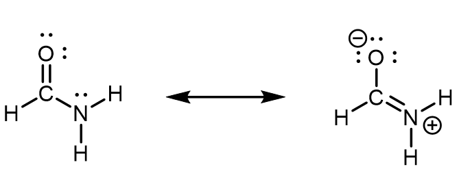
When looking at the left resonance structure, you might be tempted to assign sp 3 hybridization to N given its similarity to ammonia (NH 3 ). However, this is a resonance structure; the set of resonance structures describes a molecule that cannot be described correctly by a single Lewis structure. All atoms must remain in the same positions from one resonance structure to another in a set of resonance structures. There cannot be a N atom that is trigonal pyramidal in one resonance structure and trigonal planar in another resonance structure, because the atoms attached to the N would have to change positions.
Experimental evidence and quantum mechanics calculations show that formamide is a planar molecule, hence, the hybridization and geometry assignments are valid. This also means that the planar geometry must be more stable than the geometry involving a trigonal pyramidal sp 3 N. In other words, participation in the π bonding stabilizes the sp 2 hybridization of N.
Activity: Molecular Structure of Resonance Hybrid
Chemistry 109 Fall 2021 Copyright © by John Moore; Jia Zhou; and Etienne Garand is licensed under a Creative Commons Attribution-NonCommercial-ShareAlike 4.0 International License , except where otherwise noted.
Home / How To Determine Hybridization: A Shortcut
Bonding, Structure, and Resonance
By James Ashenhurst
- How To Determine Hybridization: A Shortcut
Last updated: December 28th, 2022 |
A Shortcut For Determining The Hybridization Of An Atom In A Molecule
Here’s a shortcut for how to determine the hybridization of an atom in a molecule that will work in at least 95% of the cases you see in Org 1.
For a given atom:
- Count the number of atoms connected to it (atoms – not bonds!)
- Count the number of lone pairs attached to it.
- Add these two numbers together.
- If it’s 4 , your atom is sp 3 .
- If it’s 3 , your atom is sp 2 .
- If it’s 2 , your atom is sp.
(If it’s 1, it’s probably hydrogen!)
The main exception is atoms with lone pairs that are adjacent to pi bonds, which we’ll discuss in detail below.
Table of Contents
- Some Simple Worked Examples Of The Hybridization Shortcut
- How To Determine Hybridization Of An Atom: Two Exercises
- Are There Any Exceptions?
- Exception #1: Lone Pairs Adjacent To Pi-bonds
- Lone Pairs In P-Orbitals (Versus Hybrid Orbitals) Have Better Orbital Overlap With Adjacent Pi Systems
- Exception #2. Geometric Constraints
- “Geometry Determines Hybridization, Not The Other Way Around”
1. Some Simple Worked Examples Of The Hybridization Shortcut
sp 3 hybridization : sum of attached atoms + lone pairs = 4
sp 2 hybridization : sum of attached atoms + lone pairs = 3
sp hybridization : sum of attached atoms + lone pairs = 2
Where it can start to get slightly tricky is in dealing with line diagrams containing implicit (“hidden”) hydrogens and lone pairs.
Chemists like time-saving shortcuts just as much as anybody else, and learning to quickly interpret line diagrams is as fundamental to organic chemistry as learning the alphabet is to written English.
- Just because lone pairs aren’t drawn in on oxygen, nitrogen, and fluorine doesn’t mean they’re not there.
- Assume a full octet for C, N, O, and F with the following one exception: a positive charge on carbon indicates that there are only six electrons around it. [ Nitrogen and oxygen bearing a formal charge of +1 still have full octets].
[ Advanced: Note 1 covers how to determine the hybridization of atoms in some weird cases like free radicals, carbenes and nitrenes ]
2. How To Determine Hybridization Of An Atom: Two Exercises
Here’s an exercise. Try picking out the hybridization of the atoms in this highly poisonous molecule made by the frog in funky looking pyjamas, below right.
[Don’t worry if the molecule looks a little crazy: just focus on the individual atoms that the arrows point to (A, B, C, D, E). A and B especially. If you haven’t mastered line diagrams yet ( and “hidden” hydrogens ) maybe get some more practice and come back to this later.]
Here are some more examples.
More practice quizzes for hybridization can be found here (MOC Membership unlocks them all)
3. Are There Any Exceptions?
Sure. Although as with many things, explaining the shortcut takes about 2 minutes, while explaining the exceptions takes about 10 times longer.
Helpfully, these exceptions fall into two main categories. It should be noted that by the time your course explains why these examples are exceptions, it will likely have moved far beyond hybridization.
Bottom line: these probably won’t be found on your first midterm.
4. Exception #1: Lone Pairs Adjacent To Pi-bonds
The main exception is for atoms bearing lone pairs that are adjacent to pi bonds.
Quick shortcut: Lone pairs adjacent to pi-bonds (and pi-systems) tend to be in unhybridized p orbitals, rather than in hybridized sp n orbitals.
This is most common for nitrogen and oxygen .
In the cases below, a nitrogen or oxygen that we might expect to be sp 3 hybridized is actually sp 2 hybridized (trigonal planar).
Why? The quick answer is that lowering of energy from conjugation of the p-orbital with the adjacent pi-bond more than compensates for the rise in energy due to greater electron-pair repulsion for sp 2 versus sp 3
[see this post: “ Conjugation and Resonance “]
What’s the long answer?
5. Lone Pairs In P-Orbitals (Versus Hybrid Orbitals) Have Better Orbital Overlap With Adjacent Pi Systems
Let’s think back to why atoms hybridize in the first place: minimization of electron-pair repulsion.
For a primary amine like methylamine, adoption of a tetrahedral (sp 3 ) geometry by nitrogen versus a trigonal planar (sp 2 ) geometry is worth about 5 kcal/mol [roughly 20 kJ/mol].
That might not sound like a lot, but for two species in equilibrium, a difference of 5 kcal/mol in energy represents a ratio of about 4400:1 ] . [How do we know this? See this (advanced) Note 2 on nitrogen inversion]
What if there was some compensating effect whereby a lone pair unhybridized p-orbital was actually more stable than if it was in a hybridized orbital?
This turns out to be the case in many situations where the lone pair is adjacent to a pi bond! The most common and important example is that of amides , which constitute the linkages between amino acids. The nitrogen in amides is planar (sp 2 ), not trigonal pyramidal (sp 3 ), as proven by x-ray crystallography.
The difference in energy varies widely, but a typical value is about 10 kcal/mol favouring the trigonal planar geometry. [We know this because many amides have a measurable barrier to rotation a topic we also talked about in the Conjugation and Resonance post]
Why is trigonal planar geometry favoured here? Better orbital overlap of the p orbital with the pi bond vs. the (hybridized) sp 3 orbital .
You can think of this as leading to a stronger “partial” C–N bond. Two important consequences of this interaction are restricted rotation in amides, as well as the fact that acid reacts with amides on the oxygen, not the nitrogen lone pair (!)
The oxygen in esters and enols is also also sp 2 hybridized, as is the nitrogen in enamines and countless other examples.
As you will likely see in Org 2, some of the most dramatic cases are those where the “de-hybridized” lone pair participates in an aromatic system . Here, the energetic compensation for a change in hybridization from sp 3 to sp 2 can be very great indeed – more than 20 kcal/mol in some cases.
For this reason, the most basic site of pyrrole is not the nitrogen lone pair, but on the carbon (C-2) (!).
6. Exception #2. Geometric Constraints
Another example where the actual hybridization differs from what we might expect from the shortcut is in cases with geometric constraints. For instance in the phenyl cation below, the indicated carbon is attached two two atoms and zero lone pairs.
What’s the hybridization?
From our shortcut, we might expect the hybridization to be sp .
In fact, the geometry around the atom is much closer to sp 2 . That’s because the angle strain adopting the linear (sp) geometry would lead to far too much angle strain to be a stable molecule.
7. “Geometry Determines Hybridization, Not The Other Way Around”
A quote passed on to me from Matt seems appropriate:
“Geometry determines hybridization, not the other way around”
Well, that’s probably more than you wanted to know about how to determine the hybridization of atoms.
Suffice to say, any post from this site that contains shortcut in the title is a sure fire-bet to have over 1000 words and >10 figures.
Thanks to Matt Pierce of Organic Chemistry Solutions for important contributions to this post. Ask Matt about scheduling an online tutoring session here .
Related Articles
- Hidden Hydrogens, Hidden Lone Pairs, Hidden Counterions
- Hybrid Orbitals and Hybridization
- How Do We Know Methane (CH4) Is Tetrahedral?
- Orbital Hybridization And Bond Strengths
- Conjugation And Resonance In Organic Chemistry
- Bond Hybridization Practice (MOC Membership)
Note 1. Some weird cases.
Sometimes you might be asked to determine the hybridization of free radicals and of carbenes (or nitrenes)
Although you’re unlikely to encounter these, let’s still have a look.
- Free radicals exist in a shallow pyramidal geometry, not purely sp 2 or sp 3 .
- However, if they are adjacent to a pi system (e.g. a C-C double or triple bond) then the shallow pyramid will re-hybridize to give it an sp 2 geometry, which allows for full resonance delocalization of the free radical.
- Carbenes and nitrenes would give us sp 2 geometry by the hybridization shortcut. However their actual structures can vary depending on whether or not the electron pair exists in a single orbital (a singlet carbene) or is divided into two singly-filled orbitals (a triplet carbene). That’s really beyond the scope of introductory organic chemistry.
What about higher block elements like sulfur and phosphorus?
Third row elements like phosphorus and sulfur can exceed an octet of electrons by incorporating d-orbitals in the hybrid. This is more in the realm of inorganic chemistry so I don’t really want to discuss it. Here’s an example for the hybridization of SF 4 from elsewhere . (sp 3 d orbitals).
Note 2 : For the 5 kcal/mol figure, see here . [Tetrahedron Lett, 1971, 37 , 3437]. (Kurt Mislow, RIP . )
An amine connected to three different substituents (R 1 R 2 and R 3 ) should be chiral, since it has in total 4 different substituents (including the lone pair). However, all early attempts to prepare enantiomerically pure amines met with failure. It was later found that amines undergo inversion at room temperature, like an umbrella being forced inside-out by a strong wind.
In the transition state for inversion the nitrogen is trigonal planar. One can thus calculate the difference in energy between the sp 3 and sp 2 geometries by measuring the activation barrier for this process (see ref ).
Note 3 :A fun counter-example might be Coelenterazine .
One would not expect both nitrogen atoms to be sp 2 hybridized, because that would lead to a cyclic, flat, conjugated system with 8 pi electrons : in other words, antiaromatic. I can’t find a crystal structure of the core molecule to confirm (but would welcome any additional information!)
NOTE – (added afterwards) If you draw the resonance form where the nitrogen lone pair forms a pi bond with the carbonyl carbon, then the ring system has 10 electrons and would therefore be “aromatic”.
- Barrier to pyramidal inversion of nitrogen in dibenzylmethylamine Michael J. S. Dewar and W. Brian Jennings Journal of the American Chemical Society 1971 93 (2), 401-403 DOI: 10.1021/ja00731a016
Pyramidal inversion barriers: the significance of ground state geometry Joseph Stackhouse, Raymond D.Baechler, Kurt Mislow Tetrahedron Letters Volume 12, Issue 37, 1971 , Pages 3437-3440 DOI: doi.org/10.1016/S0040-4039(01)97199-0
00 General Chemistry Review
- Lewis Structures
- Ionic and Covalent Bonding
- Chemical Kinetics
- Chemical Equilibria
- Valence Electrons of the First Row Elements
- How Concepts Build Up In Org 1 ("The Pyramid")
01 Bonding, Structure, and Resonance
- Sigma bonds come in six varieties: Pi bonds come in one
- A Key Skill: How to Calculate Formal Charge
- The Four Intermolecular Forces and How They Affect Boiling Points
- 3 Trends That Affect Boiling Points
- How To Use Electronegativity To Determine Electron Density (and why NOT to trust formal charge)
- Introduction to Resonance
- How To Use Curved Arrows To Interchange Resonance Forms
- Evaluating Resonance Forms (1) - The Rule of Least Charges
- How To Find The Best Resonance Structure By Applying Electronegativity
- Evaluating Resonance Structures With Negative Charges
- Evaluating Resonance Structures With Positive Charge
- Exploring Resonance: Pi-Donation
- Exploring Resonance: Pi-acceptors
- In Summary: Evaluating Resonance Structures
- Drawing Resonance Structures: 3 Common Mistakes To Avoid
- How to apply electronegativity and resonance to understand reactivity
- Bond Hybridization Practice
- Structure and Bonding Practice Quizzes
- Resonance Structures Practice
02 Acid Base Reactions
- Introduction to Acid-Base Reactions
- Acid Base Reactions In Organic Chemistry
- The Stronger The Acid, The Weaker The Conjugate Base
- Walkthrough of Acid-Base Reactions (3) - Acidity Trends
- Five Key Factors That Influence Acidity
- Acid-Base Reactions: Introducing Ka and pKa
- How to Use a pKa Table
- The pKa Table Is Your Friend
- A Handy Rule of Thumb for Acid-Base Reactions
- Acid Base Reactions Are Fast
- pKa Values Span 60 Orders Of Magnitude
- How Protonation and Deprotonation Affect Reactivity
- Acid Base Practice Problems
03 Alkanes and Nomenclature
- Meet the (Most Important) Functional Groups
- Condensed Formulas: Deciphering What the Brackets Mean
- Don't Be Futyl, Learn The Butyls
- Primary, Secondary, Tertiary, Quaternary In Organic Chemistry
- Branching, and Its Affect On Melting and Boiling Points
- The Many, Many Ways of Drawing Butane
- Wedge And Dash Convention For Tetrahedral Carbon
- Common Mistakes in Organic Chemistry: Pentavalent Carbon
- Table of Functional Group Priorities for Nomenclature
- Summary Sheet - Alkane Nomenclature
- Organic Chemistry IUPAC Nomenclature Demystified With A Simple Puzzle Piece Approach
- Boiling Point Quizzes
- Organic Chemistry Nomenclature Quizzes
04 Conformations and Cycloalkanes
- Staggered vs Eclipsed Conformations of Ethane
- Conformational Isomers of Propane
- Newman Projection of Butane (and Gauche Conformation)
- Introduction to Cycloalkanes (1)
- Geometric Isomers In Small Rings: Cis And Trans Cycloalkanes
- Calculation of Ring Strain In Cycloalkanes
- Cycloalkanes - Ring Strain In Cyclopropane And Cyclobutane
- Cyclohexane Conformations
- Cyclohexane Chair Conformation: An Aerial Tour
- How To Draw The Cyclohexane Chair Conformation
- The Cyclohexane Chair Flip
- The Cyclohexane Chair Flip - Energy Diagram
- Substituted Cyclohexanes - Axial vs Equatorial
- Ranking The Bulkiness Of Substituents On Cyclohexanes: "A-Values"
- Cyclohexane Chair Conformation Stability: Which One Is Lower Energy?
- Fused Rings - Cis-Decalin and Trans-Decalin
- Naming Bicyclic Compounds - Fused, Bridged, and Spiro
- Bredt's Rule (And Summary of Cycloalkanes)
- Newman Projection Practice
- Cycloalkanes Practice Problems
05 A Primer On Organic Reactions
- The Most Important Question To Ask When Learning a New Reaction
- Learning New Reactions: How Do The Electrons Move?
- The Third Most Important Question to Ask When Learning A New Reaction
- 7 Factors that stabilize negative charge in organic chemistry
- 7 Factors That Stabilize Positive Charge in Organic Chemistry
- Nucleophiles and Electrophiles
- Curved Arrows (for reactions)
- Curved Arrows (2): Initial Tails and Final Heads
- Nucleophilicity vs. Basicity
- The Three Classes of Nucleophiles
- What Makes A Good Nucleophile?
- What makes a good leaving group?
- 3 Factors That Stabilize Carbocations
- Equilibrium and Energy Relationships
- What's a Transition State?
- Hammond's Postulate
- Learning Organic Chemistry Reactions: A Checklist (PDF)
- Introduction to Free Radical Substitution Reactions
- Introduction to Oxidative Cleavage Reactions
06 Free Radical Reactions
- Bond Dissociation Energies = Homolytic Cleavage
- Free Radical Reactions
- 3 Factors That Stabilize Free Radicals
- What Factors Destabilize Free Radicals?
- Bond Strengths And Radical Stability
- Free Radical Initiation: Why Is "Light" Or "Heat" Required?
- Initiation, Propagation, Termination
- Monochlorination Products Of Propane, Pentane, And Other Alkanes
- Selectivity In Free Radical Reactions
- Selectivity in Free Radical Reactions: Bromination vs. Chlorination
- Halogenation At Tiffany's
- Allylic Bromination
- Bonus Topic: Allylic Rearrangements
- In Summary: Free Radicals
- Synthesis (2) - Reactions of Alkanes
- Free Radicals Practice Quizzes
07 Stereochemistry and Chirality
- Types of Isomers: Constitutional Isomers, Stereoisomers, Enantiomers, and Diastereomers
- How To Draw The Enantiomer Of A Chiral Molecule
- How To Draw A Bond Rotation
- Introduction to Assigning (R) and (S): The Cahn-Ingold-Prelog Rules
- Assigning Cahn-Ingold-Prelog (CIP) Priorities (2) - The Method of Dots
- Enantiomers vs Diastereomers vs The Same? Two Methods For Solving Problems
- Assigning R/S To Newman Projections (And Converting Newman To Line Diagrams)
- How To Determine R and S Configurations On A Fischer Projection
- The Meso Trap
- Optical Rotation, Optical Activity, and Specific Rotation
- Optical Purity and Enantiomeric Excess
- What's a Racemic Mixture?
- Chiral Allenes And Chiral Axes
- Stereochemistry Practice Problems and Quizzes
08 Substitution Reactions
- Introduction to Nucleophilic Substitution Reactions
- Walkthrough of Substitution Reactions (1) - Introduction
- Two Types of Nucleophilic Substitution Reactions
- The SN2 Mechanism
- Why the SN2 Reaction Is Powerful
- The SN1 Mechanism
- The Conjugate Acid Is A Better Leaving Group
- Comparing the SN1 and SN2 Reactions
- Polar Protic? Polar Aprotic? Nonpolar? All About Solvents
- Steric Hindrance is Like a Fat Goalie
- Common Blind Spot: Intramolecular Reactions
- The Conjugate Base is Always a Stronger Nucleophile
- Substitution Practice - SN1
- Substitution Practice - SN2
09 Elimination Reactions
- Elimination Reactions (1): Introduction And The Key Pattern
- Elimination Reactions (2): The Zaitsev Rule
- Elimination Reactions Are Favored By Heat
- Two Elimination Reaction Patterns
- The E1 Reaction
- The E2 Mechanism
- E1 vs E2: Comparing the E1 and E2 Reactions
- Antiperiplanar Relationships: The E2 Reaction and Cyclohexane Rings
- Bulky Bases in Elimination Reactions
- Comparing the E1 vs SN1 Reactions
- Elimination (E1) Reactions With Rearrangements
- E1cB - Elimination (Unimolecular) Conjugate Base
- Elimination (E1) Practice Problems And Solutions
- Elimination (E2) Practice Problems and Solutions
10 Rearrangements
- Introduction to Rearrangement Reactions
- Rearrangement Reactions (1) - Hydride Shifts
- Carbocation Rearrangement Reactions (2) - Alkyl Shifts
- Pinacol Rearrangement
- The SN1, E1, and Alkene Addition Reactions All Pass Through A Carbocation Intermediate
11 SN1/SN2/E1/E2 Decision
- Identifying Where Substitution and Elimination Reactions Happen
- Deciding SN1/SN2/E1/E2 (1) - The Substrate
- Deciding SN1/SN2/E1/E2 (2) - The Nucleophile/Base
- SN1 vs E1 and SN2 vs E2 : The Temperature
- Deciding SN1/SN2/E1/E2 - The Solvent
- Wrapup: The Key Factors For Determining SN1/SN2/E1/E2
- Alkyl Halide Reaction Map And Summary
- SN1 SN2 E1 E2 Practice Problems
12 Alkene Reactions
- E and Z Notation For Alkenes (+ Cis/Trans)
- Alkene Stability
- Alkene Addition Reactions: "Regioselectivity" and "Stereoselectivity" (Syn/Anti)
- Stereoselective and Stereospecific Reactions
- Hydrohalogenation of Alkenes and Markovnikov's Rule
- Hydration of Alkenes With Aqueous Acid
- Rearrangements in Alkene Addition Reactions
- Halogenation of Alkenes and Halohydrin Formation
- Oxymercuration Demercuration of Alkenes
- Hydroboration Oxidation of Alkenes
- m-CPBA (meta-chloroperoxybenzoic acid)
- OsO4 (Osmium Tetroxide) for Dihydroxylation of Alkenes
- Palladium on Carbon (Pd/C) for Catalytic Hydrogenation of Alkenes
- Cyclopropanation of Alkenes
- A Fourth Alkene Addition Pattern - Free Radical Addition
- Alkene Reactions: Ozonolysis
- Summary: Three Key Families Of Alkene Reaction Mechanisms
- Synthesis (4) - Alkene Reaction Map, Including Alkyl Halide Reactions
- Alkene Reactions Practice Problems
13 Alkyne Reactions
- Acetylides from Alkynes, And Substitution Reactions of Acetylides
- Partial Reduction of Alkynes With Lindlar's Catalyst
- Partial Reduction of Alkynes With Na/NH3 To Obtain Trans Alkenes
- Alkyne Hydroboration With "R2BH"
- Hydration and Oxymercuration of Alkynes
- Hydrohalogenation of Alkynes
- Alkyne Halogenation: Bromination, Chlorination, and Iodination of Alkynes
- Alkyne Reactions - The "Concerted" Pathway
- Alkenes To Alkynes Via Halogenation And Elimination Reactions
- Alkynes Are A Blank Canvas
- Synthesis (5) - Reactions of Alkynes
- Alkyne Reactions Practice Problems With Answers
14 Alcohols, Epoxides and Ethers
- Alcohols - Nomenclature and Properties
- Alcohols Can Act As Acids Or Bases (And Why It Matters)
- Alcohols - Acidity and Basicity
- The Williamson Ether Synthesis
- Ethers From Alkenes, Tertiary Alkyl Halides and Alkoxymercuration
- Alcohols To Ethers via Acid Catalysis
- Cleavage Of Ethers With Acid
- Epoxides - The Outlier Of The Ether Family
- Opening of Epoxides With Acid
- Epoxide Ring Opening With Base
- Making Alkyl Halides From Alcohols
- Tosylates And Mesylates
- PBr3 and SOCl2
- Elimination Reactions of Alcohols
- Elimination of Alcohols To Alkenes With POCl3
- Alcohol Oxidation: "Strong" and "Weak" Oxidants
- Demystifying The Mechanisms of Alcohol Oxidations
- Protecting Groups For Alcohols
- Thiols And Thioethers
- Calculating the oxidation state of a carbon
- Oxidation and Reduction in Organic Chemistry
- Oxidation Ladders
- SOCl2 Mechanism For Alcohols To Alkyl Halides: SN2 versus SNi
- Alcohol Reactions Roadmap (PDF)
- Alcohol Reaction Practice Problems
- Epoxide Reaction Quizzes
- Oxidation and Reduction Practice Quizzes
15 Organometallics
- What's An Organometallic?
- Formation of Grignard and Organolithium Reagents
- Organometallics Are Strong Bases
- Reactions of Grignard Reagents
- Protecting Groups In Grignard Reactions
- Synthesis Problems Involving Grignard Reagents
- Grignard Reactions And Synthesis (2)
- Organocuprates (Gilman Reagents): How They're Made
- Gilman Reagents (Organocuprates): What They're Used For
- The Heck, Suzuki, and Olefin Metathesis Reactions (And Why They Don't Belong In Most Introductory Organic Chemistry Courses)
- Reaction Map: Reactions of Organometallics
- Grignard Practice Problems
16 Spectroscopy
- Degrees of Unsaturation (or IHD, Index of Hydrogen Deficiency)
- Conjugation And Color (+ How Bleach Works)
- Introduction To UV-Vis Spectroscopy
- UV-Vis Spectroscopy: Absorbance of Carbonyls
- UV-Vis Spectroscopy: Practice Questions
- Bond Vibrations, Infrared Spectroscopy, and the "Ball and Spring" Model
- Infrared Spectroscopy: A Quick Primer On Interpreting Spectra
- IR Spectroscopy: 4 Practice Problems
- 1H NMR: How Many Signals?
- Homotopic, Enantiotopic, Diastereotopic
- Diastereotopic Protons in 1H NMR Spectroscopy: Examples
- C13 NMR - How Many Signals
- Liquid Gold: Pheromones In Doe Urine
- Natural Product Isolation (1) - Extraction
- Natural Product Isolation (2) - Purification Techniques, An Overview
- Structure Determination Case Study: Deer Tarsal Gland Pheromone
17 Dienes and MO Theory
- What To Expect In Organic Chemistry 2
- Are these molecules conjugated?
- Bonding And Antibonding Pi Orbitals
- Molecular Orbitals of The Allyl Cation, Allyl Radical, and Allyl Anion
- Pi Molecular Orbitals of Butadiene
- Reactions of Dienes: 1,2 and 1,4 Addition
- Thermodynamic and Kinetic Products
- More On 1,2 and 1,4 Additions To Dienes
- s-cis and s-trans
- The Diels-Alder Reaction
- Cyclic Dienes and Dienophiles in the Diels-Alder Reaction
- Stereochemistry of the Diels-Alder Reaction
- Exo vs Endo Products In The Diels Alder: How To Tell Them Apart
- HOMO and LUMO In the Diels Alder Reaction
- Why Are Endo vs Exo Products Favored in the Diels-Alder Reaction?
- Diels-Alder Reaction: Kinetic and Thermodynamic Control
- The Retro Diels-Alder Reaction
- The Intramolecular Diels Alder Reaction
- Regiochemistry In The Diels-Alder Reaction
- The Cope and Claisen Rearrangements
- Electrocyclic Reactions
- Electrocyclic Ring Opening And Closure (2) - Six (or Eight) Pi Electrons
- Diels Alder Practice Problems
- Molecular Orbital Theory Practice
18 Aromaticity
- Introduction To Aromaticity
- Rules For Aromaticity
- Huckel's Rule: What Does 4n+2 Mean?
- Aromatic, Non-Aromatic, or Antiaromatic? Some Practice Problems
- Antiaromatic Compounds and Antiaromaticity
- The Pi Molecular Orbitals of Benzene
- The Pi Molecular Orbitals of Cyclobutadiene
- Frost Circles
- Aromaticity Practice Quizzes
19 Reactions of Aromatic Molecules
- Electrophilic Aromatic Substitution: Introduction
- Activating and Deactivating Groups In Electrophilic Aromatic Substitution
- Electrophilic Aromatic Substitution - The Mechanism
- Ortho-, Para- and Meta- Directors in Electrophilic Aromatic Substitution
- Understanding Ortho, Para, and Meta Directors
- Why are halogens ortho- para- directors?
- Disubstituted Benzenes: The Strongest Electron-Donor "Wins"
- Electrophilic Aromatic Substitutions (1) - Halogenation of Benzene
- Electrophilic Aromatic Substitutions (2) - Nitration and Sulfonation
- EAS Reactions (3) - Friedel-Crafts Acylation and Friedel-Crafts Alkylation
- Intramolecular Friedel-Crafts Reactions
- Nucleophilic Aromatic Substitution (NAS)
- Nucleophilic Aromatic Substitution (2) - The Benzyne Mechanism
- Reactions on the "Benzylic" Carbon: Bromination And Oxidation
- The Wolff-Kishner, Clemmensen, And Other Carbonyl Reductions
- More Reactions on the Aromatic Sidechain: Reduction of Nitro Groups and the Baeyer Villiger
- Aromatic Synthesis (1) - "Order Of Operations"
- Synthesis of Benzene Derivatives (2) - Polarity Reversal
- Aromatic Synthesis (3) - Sulfonyl Blocking Groups
- Birch Reduction
- Synthesis (7): Reaction Map of Benzene and Related Aromatic Compounds
- Aromatic Reactions and Synthesis Practice
- Electrophilic Aromatic Substitution Practice Problems
20 Aldehydes and Ketones
- What's The Alpha Carbon In Carbonyl Compounds?
- Nucleophilic Addition To Carbonyls
- Aldehydes and Ketones: 14 Reactions With The Same Mechanism
- Sodium Borohydride (NaBH4) Reduction of Aldehydes and Ketones
- Grignard Reagents For Addition To Aldehydes and Ketones
- Wittig Reaction
- Hydrates, Hemiacetals, and Acetals
- Imines - Properties, Formation, Reactions, and Mechanisms
- All About Enamines
- Breaking Down Carbonyl Reaction Mechanisms: Reactions of Anionic Nucleophiles (Part 2)
- Aldehydes Ketones Reaction Practice
21 Carboxylic Acid Derivatives
- Nucleophilic Acyl Substitution (With Negatively Charged Nucleophiles)
- Addition-Elimination Mechanisms With Neutral Nucleophiles (Including Acid Catalysis)
- Basic Hydrolysis of Esters - Saponification
- Transesterification
- Proton Transfer
- Fischer Esterification - Carboxylic Acid to Ester Under Acidic Conditions
- Lithium Aluminum Hydride (LiAlH4) For Reduction of Carboxylic Acid Derivatives
- LiAlH[Ot-Bu]3 For The Reduction of Acid Halides To Aldehydes
- Di-isobutyl Aluminum Hydride (DIBAL) For The Partial Reduction of Esters and Nitriles
- Amide Hydrolysis
- Thionyl Chloride (SOCl2)
- Diazomethane (CH2N2)
- Carbonyl Chemistry: Learn Six Mechanisms For the Price Of One
- Making Music With Mechanisms (PADPED)
- Carboxylic Acid Derivatives Practice Questions
22 Enols and Enolates
- Keto-Enol Tautomerism
- Enolates - Formation, Stability, and Simple Reactions
- Kinetic Versus Thermodynamic Enolates
- Aldol Addition and Condensation Reactions
- Reactions of Enols - Acid-Catalyzed Aldol, Halogenation, and Mannich Reactions
- Claisen Condensation and Dieckmann Condensation
- Decarboxylation
- The Malonic Ester and Acetoacetic Ester Synthesis
- The Michael Addition Reaction and Conjugate Addition
- The Robinson Annulation
- Haloform Reaction
- The Hell–Volhard–Zelinsky Reaction
- Enols and Enolates Practice Quizzes
- The Amide Functional Group: Properties, Synthesis, and Nomenclature
- Basicity of Amines And pKaH
- 5 Key Basicity Trends of Amines
- The Mesomeric Effect And Aromatic Amines
- Nucleophilicity of Amines
- Alkylation of Amines (Sucks!)
- Reductive Amination
- The Gabriel Synthesis
- Some Reactions of Azides
- The Hofmann Elimination
- The Hofmann and Curtius Rearrangements
- The Cope Elimination
- Protecting Groups for Amines - Carbamates
- The Strecker Synthesis of Amino Acids
- Introduction to Peptide Synthesis
- Reactions of Diazonium Salts: Sandmeyer and Related Reactions
- Amine Practice Questions
24 Carbohydrates
- D and L Notation For Sugars
- Pyranoses and Furanoses: Ring-Chain Tautomerism In Sugars
- What is Mutarotation?
- Reducing Sugars
- The Big Damn Post Of Carbohydrate-Related Chemistry Definitions
- The Haworth Projection
- Converting a Fischer Projection To A Haworth (And Vice Versa)
- Reactions of Sugars: Glycosylation and Protection
- The Ruff Degradation and Kiliani-Fischer Synthesis
- Isoelectric Points of Amino Acids (and How To Calculate Them)
- Carbohydrates Practice
- Amino Acid Quizzes
25 Fun and Miscellaneous
- A Gallery of Some Interesting Molecules From Nature
- Screw Organic Chemistry, I'm Just Going To Write About Cats
- On Cats, Part 1: Conformations and Configurations
- On Cats, Part 2: Cat Line Diagrams
- On Cats, Part 4: Enantiocats
- On Cats, Part 6: Stereocenters
- Organic Chemistry Is Shit
- The Organic Chemistry Behind "The Pill"
- Maybe they should call them, "Formal Wins" ?
- Why Do Organic Chemists Use Kilocalories?
- The Principle of Least Effort
- Organic Chemistry GIFS - Resonance Forms
- Reproducibility In Organic Chemistry
- What Holds The Nucleus Together?
- How Reactions Are Like Music
- Organic Chemistry and the New MCAT
26 Organic Chemistry Tips and Tricks
- Common Mistakes: Formal Charges Can Mislead
- Partial Charges Give Clues About Electron Flow
- Draw The Ugly Version First
- Organic Chemistry Study Tips: Learn the Trends
- The 8 Types of Arrows In Organic Chemistry, Explained
- Top 10 Skills To Master Before An Organic Chemistry 2 Final
- Common Mistakes with Carbonyls: Carboxylic Acids... Are Acids!
- Planning Organic Synthesis With "Reaction Maps"
- Alkene Addition Pattern #1: The "Carbocation Pathway"
- Alkene Addition Pattern #2: The "Three-Membered Ring" Pathway
- Alkene Addition Pattern #3: The "Concerted" Pathway
- Number Your Carbons!
- The 4 Major Classes of Reactions in Org 1
- How (and why) electrons flow
- Grossman's Rule
- Three Exam Tips
- A 3-Step Method For Thinking Through Synthesis Problems
- Putting It Together
- Putting Diels-Alder Products in Perspective
- The Ups and Downs of Cyclohexanes
- The Most Annoying Exceptions in Org 1 (Part 1)
- The Most Annoying Exceptions in Org 1 (Part 2)
- The Marriage May Be Bad, But the Divorce Still Costs Money
- 9 Nomenclature Conventions To Know
- Nucleophile attacks Electrophile
27 Case Studies of Successful O-Chem Students
- Success Stories: How Corina Got The The "Hard" Professor - And Got An A+ Anyway
- How Helena Aced Organic Chemistry
- From a "Drop" To B+ in Org 2 – How A Hard Working Student Turned It Around
- How Serge Aced Organic Chemistry
- Success Stories: How Zach Aced Organic Chemistry 1
- Success Stories: How Kari Went From C– to B+
- How Esther Bounced Back From a "C" To Get A's In Organic Chemistry 1 And 2
- How Tyrell Got The Highest Grade In Her Organic Chemistry Course
- This Is Why Students Use Flashcards
- Success Stories: How Stu Aced Organic Chemistry
- How John Pulled Up His Organic Chemistry Exam Grades
- Success Stories: How Nathan Aced Organic Chemistry (Without It Taking Over His Life)
- How Chris Aced Org 1 and Org 2
- Interview: How Jay Got an A+ In Organic Chemistry
- How to Do Well in Organic Chemistry: One Student's Advice
- "America's Top TA" Shares His Secrets For Teaching O-Chem
- "Organic Chemistry Is Like..." - A Few Metaphors
- How To Do Well In Organic Chemistry: Advice From A Tutor
- Guest post: "I went from being afraid of tests to actually looking forward to them".
Comment section
39 thoughts on “ how to determine hybridization: a shortcut ”.
i am in love with this site….. explains so clear and good….. really man i was irritated because i was not able to understand but now i understand it just because of this site….
Sir thankyou so much for your explain , i was able to get a lot of things I couldn’t understand earlier, thanks a lot ,but I have a doubt about the last note ….how did it go from antiaromatic to aromatic in coelentrazine
- Pingback: How To Determine Hybridization: A Shortcut | Straight A Mindset
Thank you for the great post, as usual.
I think there is a typo in the first section of point 5 and its picture; the geometry is trigonal pyramidal instead of tetrahedral.
very helpful thanks a lot SIR
- Pingback: Hybridization involving s, p and d-Orbitals - Overall Science
thank youuuuu!!! your discussions really helped my laboratory report in organic chemistry which is due tomorrow. can you have a discussion about the effect of pi systems? i’m looking forward to it!
may i ask for the carbon hybridization of pentane and the effects of the pi system.
Pentane, C5H12 ? Tetrahedral carbons, sp3 hybridized
Well I don’t know what to say is was really helpful to I was able to understand it thank u very much
Hi James! Firstly, thank you so much for your explanation of hybridization! Here I have a question. It says if atom with lone pair next to pi bond, rehydridization will occur so we cannot use the instruction above. So how can we determine whether an atom with lone pair is next to pi bond. Thank you!
Hi, most familiar example would be the lone pairs on the OH group of a carboxylic acid, R-CO2H. The OH oxygen is sp2 hybridized since the lone pair is on an atom adjacent to a pi bond (i.e. the C=O pi bond). Another example would be an ester, R-CO2CH3 . In this case the lone pair on the oxygen bearing the CH3 (i.e. O-CH3) is sp2 hybridized since it is adjacent to a C=O bond. Amides, R-C(O)-NH2 have sp2-hybridized nitrogens, since the lone pair on the nitrogen is adjacent to a C=O bond. The negatively charged carbon in the “allyl anion” is sp2 hybridized. Lots more examples but these are a few.
This was a great review! I hadn’t done nitrogen hybridization in years and needed a quick refresher. Thanks!!!
Thanks Karla
How to determine the hybridisation state of N atom number 3 in this imidazole ring diagram?: https://upload.wikimedia.org/wikipedia/commons/thumb/b/b8/Imidazole_2D_numbered.svg/110px-Imidazole_2D_numbered.svg.png
Since by geometry, you would expect it to be sp2 hybridised, but there’s also an adjacent pi-bond system (C4 and C5), so you would expect it to be sp hybridised (such that the lone pair occupies p orbital and can undergo resonance with C=C pi orbital).
The art of teaching is so wonderful. Very clear and step-by-step explanations. My heartfelt thanks to you. My congratulations on continuing your service further.
I wonder what will be hybridization on carbocation of ethynylium ion or ethynyl carbocation.
Hi James, thanks for the concise and straight forward explanation of these exceptions. I’m teaching an orgo course this fall and feel better prepared to explain this to students.
Glad to hear it, CK, glad you find it helpful.
Hi! First, I’d like to say that I find your posts extremely helpful, certainly most of the tricks in organic chemistry I’ve learned in here. Reading this post and studying the subject I was thinking about the azobenzene and hydrazobenzene structures, I’d expect them to be sp2 and sp3, respectively, but since they have benzene rings connected to each nitrogen, would these hybridizations be valid?
Hello, thank you so much for the in-depth explanation. I’d just like to ask if exception #1 (Lone Pairs Adjacent To Pi-bonds) applies to N atom of HCN? It’s an example included in the first section as sp, but I would just like to clarify since the resources I’ve found are conflicting. Hehe, again thanks so much, sir! I hope you are well and safe.
The N atom of HCN is sp hybridized. One sp orbital is the C-N sigma bond, and the other has the lone pair on nitrogen. Under no conditions does the lone pair on nitrogen participate in resonance, since that would result in a nitrogen species with six electrons around it (less than an octet) which is very unstable!
What if the number of atom connected to it and the lone pair whe added is more than four, in total what do u call such type of hybridization
I would be wary of applying hybridization concepts to bonds in the 3rd row, such as sulfur, that exceed a full octet.
- Pingback: CCL4 Molecular Geometry, Lewis Structure, Hybridization, And Everything
Time saving concept
Thanks a lot for this info. I searched everywhere but could not get anything on these exceptions of hybridization.
Glad you found it helpful!
very helpful! thanks:))
Thanks for a clear explanation of why N and O atoms next to a pi bond or system would rather be sp2 hybridized. Gives me deeper insight as a non – organic chem teacher.
You are welcome Willetta. Thanks for stopping by.
Thanks again! I am finally gaining some facility at this thanks to your deep understanding coupled with your very clear writing.
Glad to hear it John. Thank you.
You, sir, are a tremendous help and credit to the profession of education. Thank you, thank you!
The 1H-NMR of coelenterazine (DOI: 10.1021/ct300356j) shows two signals at 9.13 (s, 1 H), and 6.44 (bs, 1 H), which suggests that the system is conjugated with the carbonyl making it all planar and aromatic when considering the entire bicyclic system. You can observe similar deshielding effects in, say, azulene for the protons on the 7-membered ring.
Now that I look at it again, you’re absolutely right. Thanks Victor.
“Third row elements like phosphorus and sulfur can exceed an octet of electrons by incorporating d-orbitals in the hybrid.”
This is incorrect, and was proven wrong years ago. See http://pubs.acs.org/doi/abs/10.1021/ja00273a006 and citing references therein. It’s more accurate (and more intuitive) to continue to follow the octet rule for sulfur, phosphorus, and other heavy main group elements. SF4, for example, can be represented as four equal-weight resonance structures of the form [SF3]+[F]-, giving an overall bond order of 0.75 for each S-F bond. This way, every atom follows the octet rule in each resonance structure. Of course you could always use molecular orbital theory in conjunction with symmetry-adapted linear combination of atomic orbitals, and then you wouldn’t need to deal with “expanded octets” in hypercoordinate molecules.
Yes and no. There’s nothing intrinsically wrong in the phrase itself as the “hypervalent” atoms DO use the higher orbitals to some extent. It is more to the point of what orbitals are involved in the overall bonding scheme. And no, nobody, who has at least some understanding of the concept of the hybridization, will insist that by saying that sulfur in SF4 has the sp3d hybridization will strictly mean that we have 100% involvement of 1 s, 3 p, and 1 d orbital in the bonding structure. It’s the same kind of argument we can bring when discussing, say, cyclopropanone. What is the hybridization of the carbonyl carbon there? Is it sp2? Is it sp2+? Is it sp2-? Is it somewhere in between? What about the hybridization in di-central rhenium complexes with quaternary bond? Or riddle me out, for instance, the exact iodine’s hybridization in every form of periodic acid ;) When we acknowledge the limitations of the theories we use, they are in a pretty good agreement with each other ;) And while using the MO is the best way to go, it is not what is being taught at the general chemistry or organic chemistry level, nor it is what students are facing on the test.
Leave a Reply
Your email address will not be published. Required fields are marked *
Save my name, email, and website in this browser for the next time I comment.
Notify me via e-mail if anyone answers my comment.
This site uses Akismet to reduce spam. Learn how your comment data is processed .
Hybridisation
The formation of bonds is no less than the act of courtship. Atoms come closer, attract to each other and gradually lose a little part of themselves to the other atoms . In chemistry, the study of bonding, that is, Hybridization is of prime importance. What happens to the atoms during bonding? What happens to the atomic orbitals? The answer lies in the concept of Hybridisation. Let us see!
Suggested Videos

Introducing Hybridisation
All elements around us, behave in strange yet surprising ways. The electronic configuration of these elements, along with their properties, is a unique concept to study and observe. Owing to the uniqueness of such properties and uses of an element, we are able to derive many practical applications of such elements.
When it comes to the elements around us, we can observe a variety of physical properties that these elements display. The study of hybridization and how it allows the combination of various molecules in an interesting way is a very important study in science.
Understanding the properties of hybridisation lets us dive into the realms of science in a way that is hard to grasp in one go but excellent to study once we get to know more about it. Let us get to know more about the process of hybridization, which will help us understand the properties of different elements.
You can download Hybridisation Cheat Sheet by clicking on the download button below

Browse more Topics under Chemical Bonding And Molecular Structure
- Bond Parameters
- Covalent Compounds
- Fundamentals of Chemical Bonding
- Hydrogen Bonding
- Ionic or Electrovalent Compounds
- Molecular Orbital Theory
- Polarity of Bonds
- Resonance Structures
- Valence Bond Theory
- VSEPR Theory
What is Hybridization?
Scientist Pauling introduced the revolutionary concept of hybridization in the year 1931. He described it as the redistribution of the energy of orbitals of individual atoms to give new orbitals of equivalent energy and named the process as hybridisation. In this process, the new orbitals come into existence and named as the hybrid orbitals.
Rules for Observing the Type of Hybridisation
The following rules are observed to understand the type of hybridisation in a compound or an ion.
- Calculate the total number of valence electrons .
- Calculate the number of duplex or octet OR
- Number of lone pairs of electrons
- Number of used orbital = Number of duplex or octet + Number of lone pairs of electrons
- If there is no lone pair of electrons then the geometry of orbitals and molecule is different.
Types of Hybridisation
The following are the types of hybridisation:
1) sp – Hybridisation
In such hybridisation one s- and one p-orbital are mixed to form two sp – hybrid orbitals, having a linear structure with bond angle 180 degrees. For example in the formation of BeCl 2 , first be atom comes in excited state 2s 1 2p 1 , then hybridized to form two sp – hybrid orbitals. These hybrid orbitals overlap with the two p-orbitals of two chlorine atoms to form BeCl 2
2) sp 2 – Hybridisation
In such hybridisation one s- and to p-orbitals are mixed form three sp 2 – hybrid orbitals, having a planar triangular structure with bond angle 120 degrees.
3) sp 3 – Hybridisation
In such hybridisation one s- and three p-orbitals are mixed to form four sp 3 – hybrid orbitals having a tetrahedral structure with bond angle 109 degrees 28′, that is, 109.5 degrees.

Studying the Formation of Various Molecules
4 equivalent C-H σ bonds can be made by the interactions of C-sp 3 with an H-1s
6 C-H sigma(σ) bonds are made by the interaction of C-sp 3 with H-1s orbitals and 1 C-C σ bond is made by the interaction of C-sp 3 with another C-sp 3 orbital.
3) Formation of NH 3 and H 2 O molecules
In NH 2 molecule nitrogen atom is sp 3 -hybridised and one hybrid orbital contains two electrons. Now three 1s- orbitals of three hydrogen atoms overlap with three sp 3 hybrid orbitals to form NH 3 molecule. The angle between H-N-H should be 109.5 0 but due to the presence of one occupied sp 3 -hybrid orbital the angle decreases to 107.8 0 . Hence, the bond angle in NH 3 molecule is 107.8 0 .
4) Formation of C 2 H 4 and C 2 H 2 Molecules
In C 2 H 4 molecule carbon atoms are sp 2 -hybridised and one 2p-orbital remains out to hybridisation. This forms p-bond while sp 2 –hybrid orbitals form sigma- bonds.
5) Formation of NH 3 and H 2 O Molecules by sp 2 hybridization
In H 2 O molecule, the oxygen atom is sp 3 – hybridized and has two occupied orbitals. Thus, the bond angle in the water molecule is 105.5 0 .
A Solved Question for You
Q: Discuss the rules of hybridisation. Are they important to the study of the concept as a whole?
Ans: Yes, the rules of hybridisation are very important to be studied before diving into the subject of hybridisation. Hence, these rules are essential to the understanding of the concepts of the topic. The following are the rules related to hybridisation:
- Orbitals of only a central atom would undergo hybridisation.
- The orbitals of almost the same energy level combine to form hybrid orbitals.
- The numbers of atomic orbitals mixed together are always equal to the number of hybrid orbitals.
- During hybridisation, the mixing of a number of orbitals is as per requirement.
- The hybrid orbitals scattered in space and tend to the farthest apart.
- Hybrid bonds are stronger than the non-hybridised bonds.
When you once use an orbital to build a hybrid orbital it is no longer available to hold electrons in its ‘pure’ form. You can hybridize the s – and p – orbitals in three ways.
Customize your course in 30 seconds
Which class are you in.

Chemical Bonding and Molecular Structure
- Aluminium Sulfate
- Silver Nitrate
- Hydroquinone
- Sodium Hydroxide
- Ferrous Sulphate
Leave a Reply Cancel reply
Your email address will not be published. Required fields are marked *
Download the App

- IIT JEE Study Material
Hybridization
Hybridization , in Chemistry, is defined as the concept of mixing two atomic orbitals to give rise to a new type of hybridized orbitals. This intermixing usually results in the formation of hybrid orbitals having entirely different energy, shapes, etc. The atomic orbitals of the same energy level mainly take part in hybridization. However, both fully-filled and half-filled orbitals can also take part in this process, provided they have equal energy.
Download Complete Chapter Notes of Chemical Bonding and Molecular Structure Download Now
On the other hand, we can say that the concept of hybridization is an extension of the valence bond theory, and it helps us to understand the formation of bonds, bond energies and bond lengths.
Table of Contents
- Key Features
sp Hybridization
Sp 2 hybridization, sp 3 hybridization, sp 3 d hybridization.
- sp 3 d2 Hybridization
What Is Hybridization?
Redistribution of the energy of orbitals of individual atoms to give orbitals of equivalent energy happens when two atomic orbitals combine to form a hybrid orbital in a molecule. This process is called hybridization . During the process of hybridization, the atomic orbitals of comparable energies are mixed together and mostly involves the merging of two ‘s’ orbitals or two ‘p’ orbitals or the mixing of an ‘s’ orbital with a ‘p’ orbital, as well as ‘s’ orbital with a ‘d’ orbital. The new orbitals, thus formed, are known as hybrid orbitals. More significantly, hybrid orbitals are quite useful in explaining atomic bonding properties and molecular geometry.
Let us have a quick look at the example of a carbon atom. This atom forms 4 single bonds wherein the valence-shell s orbital mixes with 3 valence-shell p orbitals. This combination leads to the formation of 4 equivalent sp 3 mixtures. They will have a tetrahedral arrangement around the carbon, which is bonded to 4 different atoms.
Hybridization Video Lesson

⇒ Also Read
- Chemical Bonding
- Molecular Orbital Theory
Key Features of Hybridization
- Atomic orbitals with equal energies undergo hybridization.
- The number of hybrid orbitals formed is equal to the number of atomic orbitals mixed.
- It is not necessary that all the half-filled orbitals must participate in hybridization. Even completely filled orbitals with slightly different energies can also participate.
- Hybridization happens only during the bond formation and not in an isolated gaseous atom.
- The shape of the molecule can be predicted if the hybridization of the molecule is known.
- The bigger lobe of the hybrid orbital always has a positive sign, while the smaller lobe on the opposite side has a negative sign.
Try this: Give the hybridization states of each of the carbon atoms in the given molecule.
- H 2 C = CH – CN
- HC ≡ C − C ≡ CH
- H 2 C = C = C = CH 2
Types of Hybridization
Based on the types of orbitals involved in mixing, the hybridization can be classified as sp 3 , sp 2 , sp, sp 3 d, sp 3 d 2 and sp 3 d 3 . Let us now discuss the various types of hybridization, along with their examples.
sp hybridization is observed when one s and one p orbital in the same main shell of an atom mix to form two new equivalent orbitals. The new orbitals formed are called sp hybridized orbitals. It forms linear molecules with an angle of 180°.
- This type of hybridization involves the mixing of one ‘s’ orbital and one ‘p’ orbital of equal energy to give a new hybrid orbital known as an sp hybridized orbital.
- The sp hybridization is also called diagonal hybridization.
- Each sp hybridized orbital has an equal amount of s and p characters – 50% s and 50% p characters.

Examples of sp Hybridization:
- All compounds of beryllium , like BeF 2 , BeH 2, BeCl 2
- All compounds of a carbon-containing triple bond, like C 2 H 2 .
sp 2 hybridization is observed when one s and two p orbitals of the same shell of an atom mix to form 3 equivalent orbitals. The new orbitals formed are called sp 2 hybrid orbitals.
- sp 2 hybridization is also called trigonal hybridization.
- It involves the mixing of one ‘s’ orbital and two ‘p’ orbitals of equal energy to give a new hybrid orbital known as sp 2 .
- A mixture of s and p orbital formed in trigonal symmetry and is maintained at 120 0 .
- All three hybrid orbitals remain in one plane and make an angle of 120° with one another. Each of the hybrid orbitals formed has a 33.33% ‘s’ character and 66.66% ‘p’ character.
- The molecules in which the central atom is linked to 3 atoms and is sp2 hybridized have a triangular planar shape.

Examples of sp 2 Hybridization
- All the compounds of Boron, i.e., BF 3 and BH 3
- All the compounds of carbon, containing a carbon-carbon double bond, Ethylene (C 2 H 4 )
When one ‘s’ orbital and 3 ‘p’ orbitals belonging to the same shell of an atom mix together to form four new equivalent orbitals, the type of hybridization is called a tetrahedral hybridization or sp 3 . The new orbitals formed are called sp 3 hybrid orbitals.
- These are directed towards the four corners of a regular tetrahedron and make an angle of 109°28’ with one another.
- The angle between the sp3 hybrid orbitals is 109.28 0
- Each sp 3 hybrid orbital has 25% s character and 75% p character.
- Examples of sp 3 hybridization are ethane (C 2 H 6 ) and methane.

sp 3 d hybridization involves the mixing of 1s orbital, 3p orbitals and 1d orbital to form 5 sp 3 d hybridized orbitals of equal energy. They have trigonal bipyramidal geometry.
- The mixture of s, p and d orbital forms trigonal bipyramidal symmetry.
- Three hybrid orbitals lie in the horizontal plane inclined at an angle of 120° to each other, known as the equatorial orbitals.
- The remaining two orbitals lie in the vertical plane at 90 degrees plane of the equatorial orbitals, known as axial orbitals.
- Example: Hybridization in phosphorus pentachloride (PCl 5 )

sp 3 d 2 Hybridization
- sp 3 d 2 hybridization has 1s, 3p and 2d orbitals, that undergo intermixing to form 6 identical sp 3 d 2 hybrid orbitals.
- These 6 orbitals are directed towards the corners of an octahedron.
- They are inclined at an angle of 90 degrees to one another.

Frequently Asked Questions on Hybridization
What are the different types of hybridization.
Based on the nature of the mixing orbitals, hybridization can be classified in the following ways:
- sp hybridization (beryllium chloride, acetylene)
- sp 2 hybridization (boron trichloride, ethylene)
- sp 3 hybridization (methane, ethane)
- sp 3 d hybridization (phosphorus pentachloride)
- sp 3 d 2 hybridization (sulphur hexafluoride)
- sp 3 d 3 hybridization (iodine heptafluoride)
⇒ Know more about VSEPR theory, its postulates and limitations
Among sp, sp 2 and sp 3 , which hybrid orbital is more electronegative?
The percentage of s character in sp, sp 2 and sp 3 hybridized carbon is 50%, 33.33%, and 25%, respectively.
⇒ Also Read:
- Hydrogen Bonding
- Covalent Bond
Due to the spherical shape of the s orbital, it is attracted evenly by the nucleus from all directions. Therefore, a hybrid orbital with more s-character will be closer to the nucleus, and thus more electronegative. Hence, the sp hybridized carbon is more electronegative than sp 2 and sp 3 .
Why is the hybrid orbital during hybridization better than its parent atoms?
The reason why a hybrid orbital is better than its parents is as follows:
- Parent s: because it is directional, unlike the s orbital.
- Parent p: because it has lower energy than p orbital.
What are hybrid orbitals?
Hybrid orbitals can be defined as the combination of standard atomic orbitals resulting in the formation of new atomic orbitals.
⇒ Check: Fajan’s Rule and Its Postulates
During hybridization, the hybrid orbitals possess different geometry of orbital arrangement and energies than the standard atomic orbitals. Also, the orbital overlap minimises the energy of the molecule. The degenerate hybrid orbitals formed from the standard atomic orbitals are as listed:
- 1s and 1 p: sp orbitals
- 1s and 2p: sp 2 orbitals
- 1s and 3p: sp 3 orbitals
- 1s, 3p, and 1d: sp 3 d orbitals
- 1s, 3p, and 2d: sp 3 d 2 orbitals
What is the difference between sp, sp 2 and sp 3 hybridization?
The sp hybridization occurs due to the mixing of one s and one p atomic orbital, the sp 2 hybridization is the mixing of one s and two p atomic orbitals, and the sp 3 hybridization is the mixing of one s and three p atomic orbitals.
What is the percentage of s and p characters in sp, sp 2 and sp 3 hybrid orbitals?
The percentage of s and p characters in sp, sp 2 and sp 3 hybrid orbitals is,
Sp: s characteristic 50% and p characteristic 50%
Sp 2 : s characteristic 33.33% and p characteristic 66.66%
Sp 3 : s characteristic 25% and p characteristic 75%
Explain the five basic shapes of hybridization.
The five basic shapes of hybridization are linear, trigonal planar, tetrahedral, trigonal bipyramidal and octahedral.
The geometry of the orbital arrangement is as follows:
- Linear: Two electron groups are involved resulting in sp hybridization; the angle between the orbitals is 180°.
- Trigonal planar: Three electron groups are involved resulting in sp 2 hybridization, and the angle between the orbitals is 120°.
- Tetrahedral: Four electron groups are involved resulting in sp 3 hybridization, and the angle between the orbitals is 109.5°.
- Trigonal bipyramidal: Five electron groups are involved resulting in sp 3 d hybridization; the angle between the orbitals is 90°, 120°.
- Octahedral: Six electron groups are involved resulting in sp 3 d 2 hybridization, and the angle between the orbitals is 90°.
Explain the sp3 hybridization in methane.
The 2s and all the three (3p) orbitals of carbon hybridize to form four sp 3 orbitals. These hybrid orbitals bond with four atoms of hydrogen through sp3-s orbital overlap resulting in CH 4 (methane). The geometry of orbital arrangement due to the minimum electron repulsion is tetrahedral.
The amide molecule looks like the sp 3 hybridized, but it is sp 2 . Why?
The general process of hybridization will change if the atom is either enclosed by two or more p orbitals or it has a lone pair to jump into a p orbital. Therefore, in the case of an amide molecule, the lone pair goes into a p orbital to have 3 adjacent parallel p orbitals (conjugation).
What results in the sp, sp 2 and sp 3 hybridization?
The sp and sp 2 hybridization results in two and one unhybridized p orbitals, respectively, whereas in the sp3 hybridization, there are no unhybridized p orbitals.
Explain the difference between molecular and hybrid orbitals.
The interactions between the atomic orbitals of two different atoms result in molecular orbitals, whereas when the atomic orbitals of the same atom interact, they form hybrid orbitals.

Put your understanding of this concept to test by answering a few MCQs. Click ‘Start Quiz’ to begin!
Select the correct answer and click on the “Finish” button Check your score and answers at the end of the quiz
Visit BYJU’S for all JEE related queries and study materials
Your result is as below
Request OTP on Voice Call
Leave a Comment Cancel reply
Your Mobile number and Email id will not be published. Required fields are marked *
Post My Comment
very useful
Thanks for such wonderful knowledge
Excellent knowledge thankyou
Very useful
Very helpful and easy to understand
Thanks for such good information
I have been interested with your presentation
Register with Aakash BYJU'S & Download Free PDFs
Register with byju's & watch live videos.
Talk to our experts
1800-120-456-456
- Hybridization

What is Hybridization?
Hybridization is a concept used in organic chemistry to explain chemical bonding in cases where the valence bond theory does not provide satisfactory clarification. This theory is especially useful to explain the covalent bonds in organic molecules.
Basically, hybridization is intermixing of atomic orbitals of different shapes and nearly the same energy to give the same number of hybrid orbitals of the same shape, equal energy and orientation such that there is minimum repulsion between these hybridized orbitals.
Types of Hybridization
There are different types of hybridization-based on the mixing of the orbitals.
sp³ hybridization: When one s orbital and three p orbital from the same shell of atom mix together to form a new equivalent orbital then this is called sp³ hybridization.
sp² hybridization: It is observed when one s orbital and two p orbitals undergo mixing of energy for equivalent orbitals.
sp hybridization: When one s and one p orbital goes in the process of mixing of energy to form a new orbital such kind of hybridization is called sp hybridization. The molecules possessing sp hybridization used to have a linear shape with an angle of 180°.
The above are three basic hybridizations along with them there are other hybridizations based on the mixing of orbitals such as sp³d hybridization, sp³d² hybridization and sp³d² hybridization.
Explanation of Hybridization Through Examples
Example 1: Consider an example of the simplest hydrocarbon molecular Methane. CH₄. According to experimental observations, the Methane molecule has 4 identical C-H bonds with equal length and equal bond energy. All the four hydrogen atoms are arranged in a manner such that the four hydrogen atoms form corners of a regular tetrahedron.

Image: Structural Formula of Methane
Based on the valence theory, a covalent bond is formed between two atoms in a molecule when there is an overlapping of half-filled atomic orbitals containing unpaired electrons. In the case of the methane molecule, we first write down the electronic configuration of each atom - C and H

Image: Electronic configuration of carbon and hydrogen for hybridization
Each carbon atom has two unpaired electrons (in the 2pₓ and 2pᵧ orbitals). Based on the valence theory, only two hydrogen molecules could be paired to the two unpaired electrons of the carbon atom and there will be a formation of only 2 C-H bonds in the molecule. This will lead to an incomplete octet in the 2nd orbital of the carbon molecule (2p z orbital is unfilled) and so the molecule should be unstable. However, we see that actually the methane molecule is extremely stable in nature and has 4 C-H bonds and not two. Thus, the valence theory doesn’t explain the covalent bond of the methane molecule.
The hybridization concept explains the formation of identical 4 C-H bonds and the tetrahedral shape of the molecule.
According to this concept, when a carbon atom reacts with a hydrogen atom, the electrons in the carbon atom initially go into an excited state as shown here:

Image: Electronic configuration of carbon in the ground state and in the excited state
Post excitation, hybridization can be imagined as the process where these 4 excited s and the p orbitals combine together to give a homogenous mixture and divide themselves into 4 identical orbitals having identical energy. These new orbitals have been termed hybridized orbitals. Since there one s orbital and 3 p orbitals have combined to form the hybrid orbital, the hybridized orbitals are called sp³ orbitals. The energy of these hybrid orbitals lie in between the energy levels of the s and the p orbitals as shown here:

Image: Formation of the hybridized orbital sp³
Each sp³ hybrid orbitals has one unpaired electron. Since these 4sp³ orbitals are identical in terms of energy, there is a tendency amongst these electrons to repel each other. To minimize the repulsion between electrons, the sp³ hybridized orbitals arrange themselves around the carbon nucleus in a tetrahedral arrangement. The resulting carbon atom is termed as sp³ hybridized carbon atom.

Image: Tetrahedral arrangement of sp³ hybridized orbital
Overlap of each of the 4sp³ orbitals of the hybridized carbon atom with the s orbital of the hydrogen atoms leads to the formation of a methane molecule. The methane molecule can be shown as:

Image: sp³-s overlapping to form C-H bonding
It can be seen from the above that there are 4 identical sp³-s overlaps forming 4 identical C-H bonds which are consistent with the observations. Moreover, since these sp³ orbitals are oriented in the form of tetrahedrons, the geometry of the methane molecule is tetrahedral.
Thus, adding the concept of hybridization to the valence theory helps to understand the bonding in the methane molecule.
Example 2: The above example of methane had sp³ hybridization formed because of hybridization of 1 s and 3 p orbitals of the carbon atom. There are other types of hybridization when there are hybrid orbitals between 2 p orbitals and 1 s orbital called sp² hybridization. In case, there are hybrid orbitals between 1 s and 1 p orbitals, it is called sp hybridization.
Let us consider the case of sp² hybridization. The structure of ethylene can be explained using the concept of sp² hybridization. The structure of the ethylene molecule observed is as:

Image: Electronic configuration of sp² orbital
Experimentally, the four carbon-hydrogen bonds in the ethylene molecule are identical and the geometry at each carbon atom in the ethylene molecule is planar trigonal.
Since the carbon atom has only 2 unpaired electrons, the valence bond theory cannot explain the formation of 4 bonds by each of the carbon atoms. Hence, we have to consider the excited state of both the carbon atoms in order that each carbon atom forms 4 bonds.
We first consider the two carbon atoms and the double bond between them.
For each of the excited carbon atoms, the one 2s orbital and two 2p orbitals (of the three 2p orbitals) form hybridization resulting in 3 hybrid orbitals called sp2 sp² orbitals. (1 s and 2 p orbitals). These 3 sp² orbitals try to be as distant from each other as possible and hence form a planar trigonal structure. The third 2p orbital in each of the carbon atoms does not participate in hybridization and remains as 2p orbital.

Image: Structural Formula of C₂H₄
Each of the three sp² hybrid orbitals and the non-hybrid 2p orbital has 1 unpaired electron. To minimize repulsion of this non-hybrid 2p orbital with the 3 sp² orbitals, the 2p orbital stands perpendicular to each of the sp² hybrid orbitals. Hence, post-hybridization, the sp 2 hybridized carbon atom looks as:

Image: sp 2 hybridized carbon atom
Each carbon atom in the ethylene molecule is bonded to two hydrogen atoms. Thus, overlap two sp²-hybridized orbitals with the 1s orbitals of two hydrogen atoms Also, the covalent C-C bond forms by overlapping of sp² orbitals of the two carbon atoms as:

Image: C-C bond forms by the overlapping of sp² orbitals
The two 2p orbitals of the carbon atoms overlap laterally to form a weak bond called a pi bond.
Thus, the ethylene molecule is said to have sp2- sp² s bonds (4 C-H bonds), one sp²-sp² bond (C-C bond) and one p-p pi bond (C-C bond).
Thus, the sp² hybridization theory explains the double bond, the trigonal planar structure in ethylene molecules.
Example 3: Similarly, for a triple bond formation, like that of an acetylene molecule, there is sp hybridization between 1 s and 1 p orbital of the carbon atom.

Image: Structural Formula of C₂H₂
Here, there are 2 C-H bonds and a triple C-C bond.
In each of the excited carbon atoms, one 2s and one 2p orbital form hybrid molecules called sp hybrid orbitals and the non-hybrid two 2p orbitals do not participate in hybridization. Because there are electron molecules in each of the orbitals, they tend to repel each other and the 2sp orbitals form a linear arrangement. The non-hybrid 2p orbital position themselves as far away as possible from each sp-hybridized orbital when perpendicular to each sp-hybridized orbital. So the resulting sp hybrid carbon atom looks like this:

Image: sp hybridization
The s orbitals of the hydrogen atom overlap with one sp hybrid orbital of each of the carbon atoms forming the 2 C-H bonds. The C-C covalent bond is formed by overlapping the sp-sp orbitals of the two-hybrid carbon atoms. In order to complete octet, the two non-hybrid 2p orbitals of each of the carbon atoms overlap laterally forming 2 pi bonds as shown:
Thus, sp hybridization explains the triple bond in acetylene molecules and the linear structure as well.
Nature of the Types of Hybridization
Hybridization as a concept helps explain the molecular structure and shapes of the molecules. The following table summarizes the shapes of the molecules:
Type Of Hybridization | Shape | Number Of Orbitals Participating In Hybridization |
sp³ | Tetrahedral | 4 (1s + 3p) |
sp² | Planar trigonal | 3(1s + 2p) |
sp | Linear | 2(1s + 1p) |
Hence, from the above text, we understand that hybridization is mathematically a concept of mixing atomic orbitals to form new hybrid orbitals suitable for the pairing of electrons to form chemical bonds in valence bond theory. Also, an entirely new orbital formed is different from its components and hence being called a hybrid orbital.
FAQs on Hybridization
1. What is hybridization?
The energy of the individual atoms' orbitals is transferred to create orbitals with equivalent energy when two atomic orbitals combine to create a hybrid orbital in a molecule . We refer to this process as hybridization . Atomic orbitals with the same energy level are principally responsible for hybridization . Hybridization , especially in organic chemistry , aids in the prediction of molecule shape.
For more information, refer to https://www.vedantu.com/chemistry/hybridization
2. Explain sp3 hybridization.
One s orbital and three p orbitals combine to generate four sp3 orbitals , each of which has a 25% s character and a 75% p character. This process is known as sp3 hybridization . Anytime an atom is surrounded by four groups of electrons , this kind of hybridization is necessary. These form an angle of 109°28' with one another and are oriented at the four corners of a typical tetrahedron.
3. Explain sp2 hybridization.
One s orbital and two p orbitals combine to generate three sp2 orbitals , each of which has 33% s character and 67% p character. This process is known as sp2 hybridization. Anytime an atom is surrounded by three groups of electrons , this kind of hybridization is necessary. Trigonal hybridization is another name for sp2 hybridization . A trigonal symmetry generated a mixture of s and p orbitals that is kept at 120 degrees.
4. Explain sp hybridization.
One s and one p orbital in the same main shell of an atom combine to generate two new equivalent orbitals, which is known as sp hybridization . The newly created orbitals are known as sp hybridized orbitals . It creates 180-degree angled linear molecules. To create a new hybrid orbital known as sp hybridized orbital , one 's' orbital and one 'p' orbital of equal energy are mixed together in this sort of hybridization .
5. under which chapter, hybridisation is covered?
Chapter 4 of the CBSE Class 11 Chemistry textbook, "Chemical Bonding and Molecular Structure," discusses hybridization. The scoring paper for the medical entrance exam is chemistry. You can find all of the Chemistry MCQ Questions here that follow the most recent curriculum. By regularly practicing with these Chemistry problems, you can enhance your topic knowledge, problem-solving abilities, and time management. Hybridization multiple-choice questions provide you the assurance you need to respond correctly to exam questions and raise your overall score.
https://www.vedantu.com/cbse/important-questions-class-11-chemistry-chapter-4
NCERT Study Material
- Search Menu
- Sign in through your institution
- Advance Articles
- Virtual Issues
- High-Impact Research Collection
- Celebrate 40 years of MBE
- Perspectives
- Discoveries
- Cover Archive
- Brief Communications
- Submission site
- Author guidelines
- Open access
- Self-archiving policy
- Reasons to submit
- About Molecular Biology and Evolution
- About the Society for Molecular Biology and Evolution
- Editorial Board
- Advertising and Corporate Services
- Journals Career Network
- Journals on Oxford Academic
- Books on Oxford Academic

Article Contents
Introduction, materials and methods, supplementary material, acknowledgments, author contributions, data availability.
- < Previous
Morphometrics and Phylogenomics of Coca ( Erythroxylum spp.) Illuminate Its Reticulate Evolution, With Implications for Taxonomy
Natalia A S Przelomska and Rudy A Diaz lead authors.
Oscar A Pérez-Escobar and Alexandre Antonelli senior authors.
- Article contents
- Figures & tables
- Supplementary Data
Natalia A S Przelomska, Rudy A Diaz, Fabio Andrés Ávila, Gustavo A Ballen, Rocío Cortés-B, Logan Kistler, Daniel H Chitwood, Martha Charitonidou, Susanne S Renner, Oscar A Pérez-Escobar, Alexandre Antonelli, Morphometrics and Phylogenomics of Coca ( Erythroxylum spp.) Illuminate Its Reticulate Evolution, With Implications for Taxonomy, Molecular Biology and Evolution , Volume 41, Issue 7, July 2024, msae114, https://doi.org/10.1093/molbev/msae114
- Permissions Icon Permissions
South American coca ( Erythroxylum coca and E. novogranatense ) has been a keystone crop for many Andean and Amazonian communities for at least 8,000 years. However, over the last half-century, global demand for its alkaloid cocaine has driven intensive agriculture of this plant and placed it in the center of armed conflict and deforestation. To monitor the changing landscape of coca plantations, the United Nations Office on Drugs and Crime collects annual data on their areas of cultivation. However, attempts to delineate areas in which different varieties are grown have failed due to limitations around identification. In the absence of flowers, identification relies on leaf morphology, yet the extent to which this is reflected in taxonomy is uncertain. Here, we analyze the consistency of the current naming system of coca and its four closest wild relatives (the “coca clade”), using morphometrics, phylogenomics, molecular clocks, and population genomics. We include name-bearing type specimens of coca's closest wild relatives E. gracilipes and E. cataractarum . Morphometrics of 342 digitized herbarium specimens show that leaf shape and size fail to reliably discriminate between species and varieties. However, the statistical analyses illuminate that rounder and more obovate leaves of certain varieties could be associated with the subtle domestication syndrome of coca. Our phylogenomic data indicate extensive gene flow involving E. gracilipes which, combined with morphometrics, supports E. gracilipes being retained as a single species. Establishing a robust evolutionary-taxonomic framework for the coca clade will facilitate the development of cost-effective genotyping methods to support reliable identification.
The expansion of humans into South America some 15,000 to 13,500 years ago ( Rothhammer and Dillehay 2009 ) was accompanied by the adoption, and sometimes domestication of native plants into human agroecosystems. One of the earliest known and most widely cultivated crops is coca ( Rury and Plowman 1983 ), taxonomically circumscribed as Erythroxylum coca Lam. and E. novogranatense (D. Morris) Hieron ( Schulz 1907 ; Plowman 1979 ), whose history of use traces back at least 8,000 years ( Dillehay et al. 2010 ). Coca was predominantly involved in the cultural evolution of societies owing to its medicinal, stimulatory, and cultural properties ( Schultes 1979 ; Plowman 1984 ), and many Andean and Amazonian communities today remain reliant on this plant ( Naranjo 1979 ; Cristancho and Vining 2004 ; Azevedo 2021 ; Vergara et al. 2022 ).
Despite many ethnobotanical and physiological studies, the taxonomic boundaries between cultivated varieties and their wild relatives in the genus Erythroxylum (family Erythroxylaceae) are poorly defined. The implications of an inadequate classification system of coca are pertinent to plantations, many of which supply local populations with leaves for medicinal and culinary uses ( Restrepo et al. 2019 ), while others are designated for the extraction of the plant's coveted alkaloid cocaine. Focused coca eradication to hamper drug trafficking, cocaine-linked deforestation, and armed conflict have become associated with the latter type of plantation in the last century ( Rincón-Ruiz and Kallis 2013 ; Dávalos et al. 2016 , 2021 ; Negret et al. 2019 ). While eradication programs have targeted many cocaine-producing plantations, they inevitably pose a threat to the Indigenous biocultural diversity of coca in the process, due to geographical proximity. In Colombia alone, 10% of illegal plantations occur in Indigenous territories ( UNODC 2023 ), and in Peru, the major cocaine production area in the valley of the Apurímac, Ene, and Mantaro Rivers (known as VRAEM in Spanish), overlaps with Indigenous lands ( Watson and Arce 2024 ). The United Nations Office on Drugs and Crime (UNODC) has been monitoring areas of coca cultivation annually since 1999 yet has limited tools for discriminating species or varieties. The development of new, reliable plant identification tools would therefore be highly valuable for better understanding the complex landscape of coca growing across South America.
The genus Erythroxylum P. Browne consists of over 270 species, of which about three-quarters are native to the American tropics ( Plowman and Hensold 2004 ; Jara-Muñoz et al. 2022 ). There are four varieties of cultivated cocas—two each in the species Erythroxylum coca (var. coca and var. ipadu Plowman) and E. novogranatense (var. novogranatense and var. truxillense [Rusby] Plowman). All of them have largely allopatric distributions in northwestern South America ( Bohm et al. 1982 ; our Fig. 1 ). The most widely cultivated species is E. coca (Huánuco coca). Its variety coca is native to wet montane forests of the eastern Andean slopes of Peru and Bolivia, whereas variety ipadu (Amazonian coca) is grown across the lowland Amazon basin. The less widely cultivated E. novogranatense has historically been grown in the dry valleys of the Cordilleras and the Sierra Nevada de Santa Marta ( Bohm et al. 1982 ), but has also recently been found in the Pacific region (Chocó and Cauca) ( UNODC 2016 ). Its variety truxillense (also known as “Trujillo coca”) is cultivated in arid regions of northwestern Peru for traditional use and is a flavoring and stimulant additive to the soft drink Coca Cola © ( Plowman 1986 ; Gootenberg 2003 ).

Morphology and geographical distribution of taxa in the coca clade. a) Bush of Erythroxylum novogranatense . b) Bush of E. coca var . coca. c) Leaves, flowers, immature flowers, and immature fruit of E. coca var. ipadu . d) Flowers of E. coca var. ipadu with potential pollinator. e) Leaves of E. gracilipes . f) Leaves of E. cataractarum . g) Immature flowers of E. cataractarum . h) Immature fruit of E. cataractarum . i) Illegal coca plantation established in the Amazonian forests of Putumayo department, Colombia. j) geographical distributions of cultivated and wild relative Erythroxylum taxa . Photos: Rocío Cortés-B. (a, b, c, d), William Ariza (e, f), and José Aguilar Cano (g, h, i).
Attribution of species status to the two broad types of cultivated coca ( Erythroxylum coca and E. novogranatense ) was undoubtedly influenced by their ethnobotanical significance, and differences between them were discerned through morphology, chemotaxonomy, and reproductive systems ( Rury 1981 ; Bohm et al. 1982 ; Plowman and Rivier 1983 ; Plowman 1986 ). A better understanding of the relationships among lineages of cultivated crops can now be gained with molecular markers ( Viruel et al. 2021 ). Recent population-level genomic work ( White et al. 2021 ) has suggested that cultivated coca is polyphyletic, with wild E. gracilipes Peyr. inferred as the closest living relative of both coca species.
As a leaf crop, selective pressures may have affected coca leaf shape and size to the point of these becoming taxonomically informative; leaf morphology can be part of the domestication syndrome ( Galindo Bonilla and Fernández-Alonso 2010 ; Arias et al. 2021 ). Indeed, leaf characteristics have been crucial in the formal taxonomy of coca ( Plowman 1979 , 1982 ), and are therefore used for coca identification in monitoring surveys (e.g. UNODC 2012 ). The leaves of cultivated coca are thought to be distinguishable from leaves of closely related, and often sympatric wild Erythroxylum species by being smaller, rounder, and softer ( Rury 1981 ; White et al. 2021 ). However, inter-grading variation across the two cultivated coca species and their wild relatives is pervasive ( Rury and Plowman 1983 ), and phenotypic plasticity additionally renders leaf morphology-based identification of individual coca leaves problematic ( Rury 1981 ; Rury and Plowman 1983 ). To date, rigorous statistical analyses are lacking.
Here, we investigate genetic relationships in the coca clade, assess their degree of correspondence with currently accepted taxa, and examine the discriminatory power of leaf morphology in identifying species and varieties using digitized herbarium specimens. We employ Gaussian mixture models (GMMs) to infer probabilistic morphometric clusters and assess their overlap with the currently accepted taxa. We then infer population-level nuclear and plastid phylogenies for the coca clade through a hybrid approach of genome skimming herbarium specimens and mining published Erythroxylum target capture genomic datasets. To test for gene flow among taxa, we apply phylogenetic network analysis. Finally, we apply population genomic tests to delimit population groups of coca and molecular-clock models to estimate lineage divergence times.
Leaf Size is Insufficient for Identifying the Cultivated Species and Varieties of Coca
We find that leaf size metrics have limited power to discriminate between varieties of cultivated coca and between cultivated cocas and their wild relatives. In our principal component analysis (PCA) on linear metrics, the taxa do not appear as distinct clusters. Nevertheless, PC1 does segregate most E. gracilipes individuals from the remaining taxa ( Fig. 2a ) due to the greater leaf area (loadings for area, width, and length: 0.590, 0.574, and 0.572). Leaf area is likewise significantly greater in E. foetidum compared to the remaining taxa ( t -test, P < 2.2×10 −4 ) ( Fig. 2a , supplementary figs. S1 and S4, Supplementary Material online). PC2 can be attributed to the leaf length-to-width ratio (loadings: −0.73 and 0.68 respectively, loading of area: 0.04). We note the taxonomic signal for length-to-width ratio, supported to an extent by diverging slopes for different taxonomic groups on a locally estimated scatterplot smoothing plot ( supplementary fig. S5, Supplementary Material online). Erythroxylum novogranatense var. truxillense has longer, narrower leaves than those observed in E. novogranatense var. novogranatense ( Fig. 2 ). Erythroxylum coca in turn has slightly larger leaves ( Fig. 2 , supplementary fig. S6, Supplementary Material online). However, the varietal groups of E. novogranatense and E. coca , collectively with E. cataractarum , exhibit a large proportion of overlap in leaf size morphospace ( Fig. 2a ), precluding statistically detectable taxon identification. The E. cataractarum type specimen appears near the extreme end of its morphospace ( Fig. 2a ), and closer to the centroid of E. n novogranatense var. truxillense 's distribution.

Summary of leaf morphometric analyses, encompassing leaf size and leaf shape, based on principal dataset (261 specimens, 844 leaves total). a) Morphospace representing PCA based on linear metrics, colored by verified pre-defined taxonomic identifications. Insets are eigen-leaves computed for each taxonomic subset of the data, reconstructed using the reverse Fourier transform for the mean, and ± 1.5 standard deviations from the mean, on the first two PCs of shape variation within a species. b) Morphospace representing PCA based on linear metrics, colored by assignment resulting from the GMM clustering model. Insets are bar charts representing the number of leaves sampled, and their individual cluster assignments, grouped by pre-defined taxonomic identifications. c) Plots of the distribution of values along the first PC of the EFA PCA, representing leaf roundness, grouped by taxonomic identification. d) Plots of the distribution of values along the second PC of the EFA PCA, representing acuteness at the base or apex, grouped by taxonomic identification. E. lineolatum was omitted from the EFA shape analyses due to limited sample size.
The GMMs with the highest level of statistical support model three clusters for linear metric data, with consistent support even after downsampling to 50 leaves per taxon and inclusion of samples growing either outside of their native South American range or in cultivation ( supplementary figs. S1 to S3, Supplementary Material online). The clearest element of congruence in terms of GMM-inferred groups and taxonomy is Cluster 3, which exhibits a high degree of overlap with the data taxonomically determined as E. gracilipes ( Fig. 2a and b.v ). Cluster 2 overlaps well with leaves taxonomically assigned to E. foetidum and E. coca var. ipadu and is the most frequently assigned cluster for leaves of E. coca var. coca ( Fig. 2b.i, ii, vii ), whereas Cluster 1 is assigned to most E. novogranatense var. truxillense and is the most common classification for individuals of var. novogranatense and E. cataractarum ( Fig. 2b.iii, iv, vi ). Importantly, these clustering methods based on linear metrics fail to distinguish the three wild relative species consistently and confidently from cultivated cocas. Furthermore, linear metric-based clustering was discordant with the taxonomic groupings overall (Rand index, full dataset = 0.691, Rand index, cultivated cocas only = 0.632; supplementary table S6, Supplementary Material online).
Leaf Shape Morphometrics Illuminate Traits That Define Cultivated Species
Using a reverse Fourier transform, we directly visualize outlines of leaf shapes using the statistical framework of the PCA into which our raw leaf outline data were input ( Fig. 2a ; supplementary figs. S1E, F, S2E, F, and S3E, F, Supplementary Material online), revealing the two most defining leaf shape traits ( Fig. 2a, c and d , supplementary figs. S1 to S3 and S8, Supplementary Material online), as discussed below. PC1 describes leaf shape from obovate/orbicular to lanceolate, or “roundness” of the leaves ( Fig. 2ai–vii and c ). Erythroxylum foetidum has the roundest leaves, followed by E. coca var. ipadu and E. coca var. coca which do not differ ( t -test P = 0.096; supplementary table S5a, Supplementary Material online). E. novogranatense var. novogranatense is not highly distinctive in roundness from the two E. coca varieties ( t -test P > 0.01 for each comparison; supplementary table S5a, Supplementary Material online) whereas E. novogranatense var. truxillense is very different, having the most lanceolate leaves ( Fig. 2d ; supplementary table S5a, Supplementary Material online). PC2 describes obovate versus ovate shape of the leaves, or more specifically “acuteness at the base or apex” ( Fig. 2ai–vii and d ), where wild taxa ( E. gracilipes , E. cataractarum , and E. foetidum ) have more ovate leaves than the cultivated species grouped together ( t -test, P < 0.01 for all comparisons; supplementary table S5b, Supplementary Material online). The cultivated varieties are better characterized by obovate leaf shape, especially E. novogranatense var. truxillense ( Fig. 2d ). There is no difference of high significance ( P < 0.01) between varieties and notably, E. gracilipes is only highly significantly different from one variety: E. novogranatense var. truxillense ( supplementary table S5c, Supplementary Material online). As with the linear metric data, our GMM of the highest statistical support clusters the data into three groups (consistent after downsampling), albeit with differences in group composition. Aspects of congruence between shape and size GMM clusters ( Fig. 2b , supplementary fig. S8, Supplementary Material online) are as follows: one of the modeled groups (Cluster 3) is assigned almost exclusively to leaves from E. gracilipes individuals ( supplementary fig. S8, Supplementary Material online). The principal group to which leaves of E. foetidum are assigned (Cluster 2; supplementary fig. S8, Supplementary Material online) is in turn distinct from this. Cluster 1 is prevalent, dominating in all cultivated taxa and E. cataractarum , but also common in E. foetidum and E. gracilipes ( supplementary fig. S8, Supplementary Material online). The principal coordinate analysis (PCoA) based on mean vectors of per taxon elliptical Fourier analysis (EFA) data likewise shows how all cultivated varieties form a close cluster ( supplementary fig. S9, Supplementary Material online). Overall, there is less uniformity of taxa when grouped using shape data compared to when grouped based on linear metric data ( supplementary tables S7 and S6, Supplementary Material online respectively), and an even greater mismatch of GMM-inferred clusters to the taxonomy (Rand index, full dataset = 0.555, Rand index, cultivated cocas only = 0.425; supplementary table S7, Supplementary Material online).
Erythroxylum gracilipes Gene Flow is Pervasive and Supported by Hybrid Edges
The uniparental plastid phylogeny and the 326-gene nuclear phylogeny both underscore the complex genetic structure of paraphyletic E. gracilipes ( Fig. 3a to d ), and each genomic source places E. foetidum along with specimen Spruce 3725 as sister to the coca clade. The remaining portions of the respective phylogenies exhibit incongruence, especially in the placement of the ten E. gracilipes specimens, including the Kew (Index Herbariorum code K) isotype of E. gracilipes (Spruce 3068; supplementary table S2, Supplementary Material online). This sample is encompassed in the poorly supported E. gracilipes + E. coca clade in the nuclear tree and has an unresolved position (50% likelihood bootstrap support (LBS)) within the well-supported E. novogranatense + E. cataractarum clade in the plastid tree. The plastid PCA based on genotype likelihoods (GLs) ( Fig. 3d ) additionally demonstrates that the E. gracilipes isotype plastid shares more genetic variation with E. gracilipes samples than with plastids of other taxa.

Comparative phylogenomic and population genomic analyses of coca and wild relatives. a) ASTRAL summary species tree topology derived from 326 ML phylogenies built from nuclear genes from 25 samples of Erythroxylum , with percent quartet support indicated and gene concordance factors presented. Pie charts at nodes indicate the proportion of gene trees that support (blue), or conflict with (green, red) the species tree. Here, the green proportion of the pie chart indicates the proportion of gene trees recovering the second most frequent alternative bipartition to the species tree, and red—any other alternative conflicting bipartition. Gray represents non-informative gene trees. b) ML tree reconstructed from plastomes sequenced in 25 samples of Erythroxylum , with bootstrap support after 500 iterations indicated and bootstrap support indicated. c) Nuclear genomic PCA based on 13,643 GLs computed from 18 sequenced and 155 data-mined accessions of Erythroxylum samples. Sequenced type specimens for E. cataractarum and E. gracilipes were highlighted. d) Plastid PCA based on 4,664 GLs computed from 18 sequenced and 9 data-mined accessions of 25 Erythroxylum samples. Sequenced type specimens for E. cataractarum and E. gracilipes are highlighted in (c) and (d).
Regarding E. coca , the plastid tree suggests closely related but phylogenetically distinct coca and ipadu varieties nested within a clade of E. gracilipes + E. coca ( Fig. 3b ). In the nuclear dataset, the multispecies coalescent (MSC) ASTRAL species tree indicates that gene-tree incongruence is substantial (normalized quartet score: 0.657). Furthermore, for any given bipartition within this E. gracilipes + E. coca clade, there is a mean total of 12 gene trees supporting the bipartition with strong support and 94 gene trees conflicting with strong support ( Fig. 3a ) (mean gene concordance factor (gCF)= 0.11, mean internode certainty (IC) = 0.08, supplementary fig. S11A and B, Supplementary Material online). Within this clade, a monophyletic grouping of ipadu and coca varieties has moderate support (32 supporting trees, 78 conflicting trees, gCF = 0.27, IC = 0.28), but includes a highly supported sister status of the two coca samples (gCF = 0.91, IC = 0.86). In contrast, E. cataractarum and E. novogranatense are well-supported, monophyletic groups, each with 100% LBS in the plastid phylogeny ( Fig. 3b ) and characterized by high gene-tree support values in the ASTRAL tree ( E. cataractarum gCF = 0.82, IC = 0.86; E. novogranatense gCF = 0.83, IC = 0.87). Similar values were obtained for the concatenated RAxML species tree ( supplementary fig. S12A and B, Supplementary Material online).
The phylogenetic network analysis ( Fig. 4c ), conducted on the same set of 25 samples to gain a broader picture of the evolutionary history of the clade, provides support to the hypothesis of gene flow involving E. gracilipes. The best network suggests two reticulations. The first is highly supported (LBS = 98, credible intervals for major and minor edges 0.62 to 0.80 and 0.20 to 0.37 respectively) and originates in the same clade as the early diverging, monophyletic Ecuadorian E. gracilipes clade, with the E. gracilipes + E. coca clade as the recipient (inheritance proportion = 0.70). The second most frequent hybridization edge detected (credible intervals for major and minor edges 0.67 to 0.90 and 0.10 to 0.33 respectively) sits within the E. gracilipes + E. coca clade, and likewise involves a monophyletic E. gracilipes outgroup supplying genetic material to an ingroup including the cultivated lineages (inheritance proportion = 0.83). An alternative recipient position with lower support was recovered for this second hybridization. The main source of uncertainty in this hybridization event likely lies with the recipient branch, on the basis that the donor branch has a higher combined support (combined bootstrap support considering all alternative recipients = 76). However, since the orientation of gene flow relies on support of the minor edge in the hybridization event, and is concordant here, we consider the gene flow direction to be highly supported.
Absolute times of divergence of lineages in the coca clade based on populations. a) Chronogram representing dates of divergence within the clade currently including E. gracilipes, E. cataractarum, E. coca and E. novogranatense. E. foetidum and E. williamsii serve as successive outgroups. Consensus topology shown in dark blue. Alternative topologies in pink and green. 95% highest posterior density intervals of absolute ages indicated as shaded area and percentage support provided at each node. b) NGSadmix population structure inference showing per-individual ancestry of sequenced and data-mined accessions of 173 Erythroxylum specimens at highly supported values of K = 4 and K = 5. Full results of per-individual ancestry inference for varying values of K provided in Supplementary material online. c) Phylogenetic network demonstrating waves of gene flow (“hybrid events”). Numbers on branches represent bootstrap values lower than 100. Numbers in italics are bootstrap values for the hybridizations. Any alternative recipient positions for a hybridization event shown as a dotted line. Inheritance proportion values are presented for the optimal network. Colored numbers represent the inheritance proportions for the major (dark blue) and minor (light blue) edges, depicting their point estimates (see main text for credible intervals).
Bioculturally Important Varieties Differ in Degree of Intraspecific Genetic Differentiation
Our nuclear PCA analyses based on nuclear GLs called in the 18 sequenced specimens and 155 data-mined samples combined (hereafter, the “merged dataset”) show genetic structure within E. gracilipes . The most substantial proportion of its diversity manifests as a cluster containing the isotype of E. gracilipes (Spruce 3068) ( supplementary table S2, Supplementary Material online), corresponding to “gracilipes1” sensu White et al. (2021) ( Fig. 3c ). This group, along with a secondary E. gracilipes and a single E. cataractarum cluster, are observed in both the merged dataset ( Fig. 3c ) and in our wild relatives-focused sampling from Kew specimens only ( supplementary fig. S13, Supplementary Material online). The merged dataset PCA ( Fig. 3c ) exhibits the largest proportion of the variation as being driven by genetic differentiation between E. novogranatense and E. coca var. coca . Within E. novogranatense, the varieties novogranatense and truxillense do form separate clusters, but with more subtle differentiation. In comparison, the varieties of E. coca : var. coca, and var. ipadu are clearly distinct. Unsupervised clustering predicted the highest values of Δ K for scenarios of genetic structuring where E. novogranatense (both varieties), E. coca var . coca , E. gracilipes (containing E. coca var. ipadu ), and E. cataractarum resolve as three or four broadly separate genetic entities ( Fig. 4b , supplementary figs. S14 and S15, Supplementary Material online). The isotype-defined E. gracilipes group becomes distinct at K = 5 ( Fig. 4b ) and E. coca var. ipadu at K = 6 ( supplementary fig. S14, Supplementary Material online). Only under a model of eight hypothetical populations does E. novogranatense var. novogranatense emerge as a cluster distinct from E. novogranatense var. truxillense ( supplementary fig. S14, Supplementary Material online).
Lineage Divergence of Cultivated Cocas Long Precedes the Peopling of South America
We inferred a time-calibrated phylogeny using a Bayesian MSC approach to estimate ages of divergence within this clade. In our population-focused approach, we combined a species tree relaxed molecular-clock model with information on population membership determined using NGSadmix ( Skotte et al. 2013 ). From this, we reliably reconstructed a species tree for the coca species and varieties and inferred absolute ages of their divergence from closely related wild relatives in the presence of topological discordance ( Ogilvie et al. 2017 ). The results imply that the coca clade diversified 2.2 million years ago (Ma) (± 1 Ma, posterior probability (PP) = 1.0) ( Fig. 4a ). The cultivated cocas and their wild-living relatives shared a common ancestor ∼1.6 Ma ago (± 700 thousand years (Kyrs), PP = 1.0). The divergence of the cultivated E. novogranatense and E. coca var. coca lineages from E. cataractarum and E. gracilipes (1,400 to 800 Kyrs, PP = 0.93 and 800 to 400 Kyrs, PP = 1.0 respectively) precedes the peopling of the American tropics (∼15.5 Ka; Dillehay et al. 2008 ; Rothhammer and Dillehay 2009 ; Prates et al. 2020 ) by hundreds of millennia.
Establishing a robust taxonomy is vital for research into plants that are medicinally, nutritionally, or culturally valuable to humans (e.g. Pironon et al. 2024 ). Plant classification at this scale is often non-trivial, since it involves elucidating the plants’ evolutionary trajectories within a wider pool of genetic diversity comprising crop wild relatives, hybrids, and semi-domesticated forms ( Pellicer et al. 2018 ; Pérez-Escobar et al. 2021 , 2022 ; Simon et al. 2022 ). For coca, its naming system has a further layer of relevance, being directly linked to the existence of legal frameworks, which on one side aim to hamper trafficking, but on the other hold the possibility of promoting opportunities for local communities that depend upon coca cultivation for traditional uses.
Evolution and Reticulation of Lineages in the Coca Clade
Our new plastid tree for the coca clade corroborates the hypothesis of White et al. (2021) proposing E. gracilipes as a clade within which E. cataractarum , E. novogranatense , and E. coca are nested. Our population genomic and phylogenomic analyses which build upon this study illustrate extensive genetic structure characterizing E. gracilipes , a shrub proposed as the wild progenitor of all described varieties of cultivated coca ( Macbride 1949 ; White et al. 2021 ). It is unsurprising that a plant species with a broad geographic distribution should show non-discrete clustering ( Dodsworth et al. 2021 ) and E. gracilipes is indeed distributed widely—in wet biomes across tropical South America ( White et al. 2019 ) ( Fig. 1j ). Counteracting this structure, we find prevalent gene flow between lineages currently considered as E. gracilipes , involving both early diverging clades and the admixed E. gracilipes + E. coca clade. This differs to the findings of White et al. (2021) who conducted maximum likelihood (ML) Treemix analysis ( Pickrell and Pritchard 2012 ) to conclude that none of the three most significant waves of gene flow in the coca clade involved the poorly resolved E. gracilipes + E. coca clade, but instead featured E. cataractarum as donor or recipient of genetic material. Treemix can be biased when applied to a dataset that includes multiple admixed populations and this method warrants extra support in most scenarios ( Lipson et al. 2013 , 2020 ). Future analyses using more genomic markers will allow for the re-evaluation of all gene flow events inferred for the coca clade thus far.
The dominant E. gracilipes group, including the Spruce 3068 isotype, was previously identified as “gracilipes1” ( White et al. 2021 ), who proposed to retain it as a genetically constricted species of E. gracilipes , while re-classifying other pockets of genetic variation within E. gracilipes as separate species. While there is a clear rationale for this proposition, we believe there are reasons for considering an alternative approach. First, there is insufficient evidence that the E. gracilipes population groups are independently evolving lineages, given the shallowness of many branches on the phylogenomic trees and degree of nuclear gene-tree conflict first indicated by White et al. (2021) and supported by gene flow patterns detected in this study. As a second argument, expressed phenotypes remain highly relevant to botanical classification ( Wells et al. 2022 ) not least due to their applicability in ecological contexts such as functional diversity ( Sultan 2000 ). Rigorous phenotypic analysis, facilitated by advances in the field of morphometrics ( Christodoulou et al. 2020 ) here supports a high degree of consistency in terms of the large, mucronate to acuminate leaves of E. gracilipes . Combined with dependable characters used for taxonomy mainly based on lanceolate and coriaceous leaves, and free styles in brevistylar and longistylar flowers, this still supports the retention of a single species. Splitting of E. gracilipes could also have consequences for interpretation of the evolution of the domesticated E. novogranatense and E. coca lineages, reinforcing the idea of domestication events isolated in space and time. Such a model is incongruent with the theory of a protracted timescale of human selection on coca that spans a variety of habitats ( Plowman 1984 ), now well-supported by the landscape-level domestication paradigm, built on evidence of extensive human-mediated genetic exchange ( Allaby et al. 2022 ; Fuller et al. 2022 ).
We deduce that the gene pool ancestral to E. gracilipes encompassed rich standing genetic variation, from which lineages of E. novogranatense , E. cataractarum , and E. coca var. coca also emerged, probably in response to novel environmental and ecological conditions. Our molecular dating results showing clade divergence of the lineages of species currently regarded to be cultivated in the mid to late Pleistocene suggest that these had already undergone adaptation to ecological conditions distinct from those of their sister wild-living, forest-dwelling relatives; at the point of being selected, these populations were feasibly pre-adapted to a human environment in which they then experienced anthropogenic selection. The species E. cataractarum was mostly shaped by adaptation to drier, high-altitude habitats of the eastern Andean slopes ( White et al. 2021 ). Despite limited sampling, genomic data support monophyly of this group. There is some ethnobotanical evidence of the use of E. cataractarum ( Schultes 1981 ), including the inscription on the K-type specimen itself “Ipadú das cachocinas” (“ipadu” being an Indigenous name for coca widely used in Brazil; Plowman 1979 ). Erythroxylum cataractarum is not documented as a cultivated variety of coca but, considering the high degree of leaf morphological overlap with cultivated cocas, its use cannot be ruled out ( Plowman and Rivier 1983 ).
Erythroxylum novogranatense and E. coca var. coca have been taxonomically proposed as “neo-species” resulting from long-term human cultivation and selection ( Rury 1981 ), and the population genomic results confirm the distinctness of these taxa sensu lato . We urge caution in labeling these “independently evolving monophyletic lineages” ( White et al. 2021 ), since this is not supported by the evidence for ancient gene flow we detected across datasets and overlooks the diffuse nature of domestication ( Allaby et al. 2008 ; Gross and Olsen 2010 ). On the other hand, we agree that the differentiation is appreciable, phylogenomically supported, and one argument for retaining their respective species designations. The differentiation could have been driven in part by breeding system: the majority of Erythroxylum spp. are reportedly heterostylous ( White et al. 2019 ), with E. coca var. coca and E. novogranatense exhibiting self-incompatibility ( Ganders 1979 ). Heterostyly has previously been linked to elevated genetic differentiation between Neotropical species of Erythroxylum ( Abarca et al. 2008 ). In contrast, E. coca var. ipadu , which is the only variety of coca that is predominantly out-crossing ( Plowman 1979 ) exhibits genetic identity linked to that of the isotype-defined E. gracilipes group. This reinforces our phylogenomic conclusion—of a close genetic relationship of E. coca var. ipadu to this population of the wild E. gracilipes, which could have implications for the future taxonomic status of this variety.
Distinct Leaf Phenotypes in the Coca Clade Revealed by Morphometrics
Our leaf morphometric dataset provides evolutionary insights that complement the phylogenomic inferences, supporting multiple origins of coca as a leaf crop. Our most significant finding in this context is that of leaf size distinctness between wild E. gracilipes and smaller-leaved domesticated E. coca and E. novogranatense . E. coca var. ipadu is not excluded from this pattern, despite its close genetic affinity to E. gracilipes. Our data also show a tendency for rounder leaves in E. coca compared to wild species. Hence, we provide statistical evidence that partly supports cultivated coca leaves being smaller and rounder than those of their wild progenitor ( White et al. 2021 ), a hypothesis built upon in-depth physiological studies of stomatal density and vein morphology ( Rury 1981 ). A possible scenario partially supported by our results is that cultivated cocas are the result of evolutionarily distinct adaptations from wild forest progenitors to novel, open habitats with greater exposure to sunlight. Those habitats likely arose as a consequence of global temperature decline and climatic fluctuations following the onset of Pleistocene glaciations at c. 2.6 Ma, which led to widespread contraction of rainforests and expansion of drier habitats ( Silva et al. 2018 ). The species currently regarded as domesticated then needed to invest fewer resources into leaf expansion than they would in the moist forest habitat of E. gracilipes . Experimental work has revealed latent plasticity in leaf size within all described varieties of cultivated coca—manifested not only in smaller “sun leaves” and larger “shade leaves” not only in their native neotropical setting, but also when cultivated under glass at temperate latitudes ( Rury and Plowman 1983 ). Leaf morphology is generally evolutionarily labile in plants and thus readily adaptable to new microhabitats or biomes ( Spriggs et al. 2018 ). We propose that the consistently smaller leaves in cultivated cocas are the result of genetic canalization ( Flatt 2005 ; Piperno 2017 ), whereby phenotypic variation in the cultivated species has largely become developmentally constrained to small leaf size. A significant shift in environmental conditions, including escape from and survival outside of human cultivation, might over time unlock persistent cryptic genetic variation ( Flatt 2005 ), here responsible for the large-leaved E. gracilipes phenotype. Erythroxylum cataractarum is a highly valuable control taxon to benchmark this theory of leaf shape evolution. Having presumably circumvented the selective pressures associated with human cultivation, it has nonetheless attained a leaf size statistically indistinguishable from that of cultivated cocas.
Another possible domestication syndrome trait is acuteness at the leaf base (lending an obovate shape), which contrasts to the frequently observed apical acuteness of wild E. gracilipes . Given the sheer volume of leaves harvested by certain Indigenous communities to supply their daily needs of almost constant coca chewing ( Schultes 1981 ), it is plausible that reorganization of the leaf structure to be amenable to human leaf picking could have given these coca bushes an adaptive advantage. Interestingly, the EFA distils basal acuteness as a trait occurring in cultivated coca varieties but not in E. cataractarum. Finally, the length-to-width ratio of coca leaves could warrant further study; this has been pinpointed e.g. as the primary source of variation between accessions and species of apple, with a heritable basis ( Migicovsky et al. 2018 ).
Studies of other plants cultivated for their fruit ( Chitwood et al. 2013 ; Chitwood and Otoni 2017 ; Klein et al. 2017 ) or roots ( Gupta et al. 2020 ) have shown that leaf shape, as inferred through an EFA framework, is highly heritable. EFA has been used to demonstrate that morphological groupings are consistent with species boundaries ( Andrade et al. 2008 ; Sayıncı et al. 2015 ; Klein et al. 2017 ), but this is not consistently true across plant groups, and particularly not for domesticates occupying ecosystems more diverse than that of a modern agricultural setting ( Soares et al. 2011 ; Nascimento et al. 2021 ), which is the case for traditionally cultivated coca.
Taxonomic Implications
Synthesizing the evidence from phylogenomics, gene flow analyses, phenotypic plasticity in coca leaf shape, and the limited discriminatory power of other characters such as leaf venation and floral anatomy ( Plowman 1979 ; Rury 1981 ), a phylogenetic species concept could be applied here to lump E. gracilipes , E. coca , E. novogranatense , and E. cataractarum into a single species. Nevertheless, the insights from population genomics and molecular dating do support the identity of long-recognized, and distinct cocas. As such, we propose that the names of these are retained for the time being, so as not to compromise their cultural significance. A future prospect could entail re-classifying E. coca var. ipadu, E. coca var. coca, E. novogranatense var. novogranatense , and E. novogranatense var. truxillense as varieties of equal standing within a more complex species, to more easily accommodate any new varieties of coca that are described using genomic, ethnobotanical, and metabolomic evidence.
The challenging, subtle nature of morphological differences between cultivated cocas and their closest wild relatives first underscored by Rury (1981) supports the failure of our linear metric and EFA analyses to reliably classify coca leaves by current taxonomy. Previous attempts to discriminate Colombian coca varieties by leaf morphology have been similarly inconclusive ( Galindo Bonilla and Fernández-Alonso 2010 ; Rodríguez Zapata 2015 ). Yet, the analyses introduced here did yield statistically supported insights regarding leaf phenotypes which can be leveraged for further research of this clade. The phylogenomic evidence base we assembled can serve as a platform for further studies interrogating the complex evolutionary trajectory of lineages in the coca clade and for potential taxonomic revisions. We also hope that it will contribute to the development of sensitive genomic methods to identify species and varieties of coca and to highlight the importance of safeguarding portions of its diversity which are under the stewardship of Indigenous communities.
Leaf Morphometrics
Image preparation.
A total of 1,163 leaf outlines were extracted from 342 digital herbarium specimens, representing individuals collected in the wild (species: E. gracilipes Peyr., E. cataractarum Spruce ex. Peyr, E. lineolatum DC., and E. foetidum Plowman), as well as plants cultivated in the neotropics or under glass at temperate latitudes ( Erythroxylum coca Lam. (var. coca and var. ipadu ) and E. novogranatense (D. Morris) Hieron (var. novogranatense and var. truxillense [Rusby] Plowman) ( supplementary table S1, Supplementary Material online). Species identities of the specimens were recorded from herbarium labels. We obtained taxonomic identities directly from specimens and compared them with specimens cited in local monographs ( Pineda 2016 ), morphological characters proposed by White et al. (2021 ; supplementary table S1, Supplementary Material online), type specimens, protologs, and geographical distributions. Based on these resources, we excluded any candidate specimens that could not be confidently assigned to any Erythroxylum species of interest to this study and re-assigned the taxon for several cultivated samples ( n = 14). A balanced sampling for each specimen was always expected as input, but the number of leaves on each specimen that were both intact and fully developed was variable. Hence, we set an upper limit of five leaves and a lower limit of two leaves per specimen. A leaf was considered fully developed if it was roughly the same size as the largest leaf on the sheet and showed shape characteristics consistent with botanical descriptions. Leaves were sampled only if they were pressed flat and intact from the base to the apex.
Image features that obstructed leaf contours (e.g. herbarium tape, twigs, and cracks) were manually removed with a digital paintbrush and images were segmented to isolate selected leaves. Outlines were extracted as coordinates using the “DiaOutline” software ( Wishkerman and Hamilton 2018 ), implemented in R. Digital noise was removed from the outlines using the “coo.smooth” function in the R package “Momocs” v.1.3 ( Bonhomme et al. 2014 ). A total of 200 equidistant, non-homologous pseudo-landmarks were sampled from each outline (“coo.sample” function in “Momocs”; Bonhomme et al. 2014 ). Two additional landmarks were manually defined at homologous positions on the base and apex of every leaf (“def_ldk” function in “Momocs”; Bonhomme et al. 2014 ).
Calculating Linear Metrics and Shape Variables
Outlines were standardized to 100 pixels per centimeters and linear metrics (length, width, and area) were recorded for each leaf using the “coo_toolbox” in “Momocs” ( Bonhomme et al. 2014 ). To generate quantitative shape variables, leaf outlines were decomposed by elliptical Fourier analysis (“efourier” function in “Momocs”; Kuhl and Giardina 1982 ; Bonhomme et al. 2014 ). This type of outline analysis relies on the principle of Fourier series to express an outline as the sum of simpler trigonometric functions. The frequencies of each harmonic in the series are described by four scalar coefficients. These coefficients can be treated statistically as homologous, quantitative variables ( Zelditch et al. 2004 ; Claude 2008 ). The minimum number of harmonics necessary for ample shape reconstruction was estimated through estimation of harmonic power ( Lestrel 1997 ; Bonhomme et al. 2014 ). We computed 14 harmonics, representing a cumulative harmonic power near 100%. Because the coefficients of an elliptic Fourier descriptor are not invariant in size, rotation, shift, and starting point of chain-coding about a contour ( Yoshioka et al. 2004 ), we standardized the Fourier coefficients prior to this shape analysis. Outlines were normalized with Bookstein baseline superimposition to the two homologous landmarks defined in outline preparation (“fgProcrustes” function in “Momocs”; Friess and Baylac 2003 ; Bonhomme et al. 2014 ). The dataset was passed through a second round of normalization, as part of the default “efourier” function in “Momocs”.
Leaves with aberrant shapes heavily skew dimensionality reduction, thus we removed these from the dataset prior to further analyses. Aberrant leaf shape outliers were identified by modeling the shape variation for each species as normally distributed, with a confidence level of 1e −3 (“which_out” function in “Momocs”; Bonhomme et al. 2014 ). In total, 15 leaves with aberrant shapes were excluded. Upon inspection, aberrant contours were mostly due to distortion from the drying process.
Morphometrical Statistical Analyses
Shape and size are separate aspects of an organism's morphology, and natural patterns can be obscured if an investigation should confound the two ( Christodoulou et al. 2020 ). Therefore, we treated linear metrics and shape variables separately in statistical analyses. To define morphological spaces for respective linear metric and shape cluster analyses, data dimensionality was reduced via PCA ( Claude 2008 ). To visualize the distribution of the most common leaf shapes within a species, we performed PCA separately for each taxonomic subset of Fourier data, after which eigen-leaves were reconstructed using the reverse Fourier transform for the mean, and +/− 1.5 standard deviations from the mean, on the first two PCs of shape variation within a species (“PCcontrib” function in “Momocs”; Bonhomme et al. 2014 ). To assess the distribution of our taxon-binned leaf data along the first two axes of variation, corresponding to defining leaf traits, we constructed eigen-leaves for the first two PCs of the shape—EFA PCA, encompassing 95.4% of the variation combined ( supplementary fig. S1E, Supplementary Material online).
To investigate the question of whether underlying structure in this morphometric dataset reflects current taxonomic boundaries, variation within this dataset was examined without a priori identifications. We inferred morphological groups probabilistically using model-based clustering using GMMs ( Bouveyron and Brunet-Saumard 2014 ; Bouveyron et al. 2019 ). This method of cluster analysis assumes that continuously distributed data can be described as a mixture (weighted average) of G multivariate normal distributions (clusters). The aim is to identify the number of groups ( G ) and the geometric properties of their densities; different model parameters correspond to different hypotheses of group structure ( Bouveyron et al. 2019 ). Model selection was performed with the expectation-maximization (EM) algorithm, which estimates model parameters by maximum likelihood ( Dempster et al. 1977 ). Measures of empirical support are based on the Bayesian information criterion (BIC; ( Schwarz 1978 ), wherein Δ BIC expresses the gain in the explanatory power of the model when an additional group is considered by the algorithm. Based on Δ BIC, an EEV geometrically-constrained clustering model (ellipsoidal, equal volume, and shape) was selected for Fourier data and an EVE model (ellipsoidal, equal volume, and orientation) was selected for linear metrics. Each leaf was assigned to a cluster by soft classifications—expectations of the assignments under the applied probability model. GMMs were fitted using the “mclust” v.5.0 package ( Scrucca et al. 2016 ), with parameters set to model two to fifteen groups. If leaves are well-classified by a given model, the conditional probability that a leaf belongs to one of the postulated groups should be close to 1. To statistically quantify equivalence between taxonomic clusters and GMM-inferred clusters, we applied the Rand index, whose value indicates the degree of correspondence of two different clustering outcomes from 0 = complete mismatch 1 = to perfect match ( Rand 1971 ). We also applied the adjusted Rand index which corrects for chance ( Hubert and Arabie 1985 ), carrying out all analyses in the “Fossil” package ( Vavrek 2011 ) implemented in R.
Noisy variables in high-dimensional data are known to degrade the performance of model-based clustering, so variable selection is crucial ( Bouveyron et al. 2019 ). Only three morphological variables were recorded for leaf size, so data were relatively low-dimensional. As such, all three principal components (PC) of their log-transformation were used in cluster analysis. Although Fourier descriptors of leaf shape are more complex in dimension, experimental exploration of a modeling approach to model selection ( Maugis et al. 2009 ) did not provide valuable insight. Therefore, we retained the four PCs explaining most of the variation, deeming these most useful in defining group structure following previous studies ( Sneath and Sokal 1975 ; Ezard et al. 2010 ). To visualize clustering for each leaf on a given herbarium specimen, bar charts were created to represent the number of leaves sampled, and their individual cluster assignments ( Fig. 2b , supplementary figs. S7 and S8, Supplementary Material online).
Canonical Variants Analysis
To visualize relationships between the a priori taxonomically defined groups in morphological space, we also computed mean vectors for the shape variables. Euclidean distances between these were calculated using the R package “rdist” ( Blaser 2020 ) and the output distance matrix was used for PcoA (“pcoa” implemented in R package “ape”).
Dataset Filtering and Downsampling
Finally, we carried out four iterations of filtering our full dataset of 1,163 digitized, taxonomically verified leaf outlines from 342 specimens. The primary purpose was to produce a dataset excluding those samples assigned dubious IDs after the taxonomic evaluation and those which were cultivated outside of South America. This dataset consisted of 844 leaf outlines from 261 specimens. We reran the analyses using the filtered dataset for our main interpretation of the results. The second filtering iteration had the goal of demonstrating that there was no bias due to different sample sizes for different taxa. Therefore, for each pre-assigned taxonomic group, we downsampled to a random subset of 50 leaves (excluding E. lineolatum , for which this quota was not reached), resulting in a dataset of 335 leaves from 167 samples. The final two iterations involved retaining from our main interpretation dataset only the cultivated coca species with a main goal of computing the degree of correspondence between the taxonomic groups and GMM clusters. One of the iterations comprised the full dataset of E. coca and E. novogranatense individuals (404 samples total, 106 specimens) and the other is a subset of these, including only one leaf per specimen (97 samples total).
Taxon Sampling and Genomic Data Mining
Our taxon sampling builds upon previous phylogenomic and population genomic studies of the coca clade ( White et al. 2019 , 2021 ). We generated new data from 18 accessions of coca and its closest wild relatives, following the current taxonomy ( Plowman 1982 ; White et al. 2019 , 2021 ) and spanning a large proportion of the geographical distribution ( supplementary fig. S10, Supplementary Material online). Our sampling included 12 specimens of E. gracilipes (including a Kew (K) isotype), four of E. cataractarum (including a K holotype), one specimen of E. lineolatum , and one specimen of E. foetidum (to serve as outgroups, based on White et al. 2019 ), as well as one specimen of E. n. novogranatense (S.S. Renner 2888) ( supplementary table S2, Supplementary Material online). For each sample, we weighed out 0.2 to 0.3 g of leaf tissue and pulverized this using steel ball bearings in a SPEX sample prep tissue homogenizer (SPEX Inc, NJ, USA). We extracted genomic DNA following a CTAB protocol, with the addition of 2% v/v 2-mercaptoethanol ( Doyle and Doyle 1990 ). DNA extracts were purified using a bead clean up method with a 2:1 ratio of Ampure XP beads (Beckman Coulter, USA) to DNA eluate. DNA extracts were quantified using a Quantus fluorometer (Promega, USA) and the degree of DNA fragmentation was assessed using a 4200 TapeStation system (Agilent Technologies, USA). We conducted library preparation using a NEBNext Ultra II DNA Library Preparation Kit according to the manufacturer's protocol. Sequencing of DNA libraries was carried out on an Illumina HiSeq platform with a paired-end 150 bp configuration, by GeneWiz (South Plainfield, USA). To complement our Erythroxylum genomic dataset, we mined read data for wild relatives and cultivated species of coca from NCBIs sequence read archive (SRA) repository. This comprised raw sequence data from 155 herbarium specimens from which DNA had been extracted and enriched for 427 nuclear genes via target capture with a custom-designed set of RNA probes ( White et al. 2019 , 2021 ) (hereafter: “mined dataset”) ( supplementary table S3, Supplementary Material online). This brought the total of samples used for some downstream analyses to 173.
Processing of Raw Read Data and Alignment to Target sequences
We trimmed raw reads (both sequenced and data-mined) using AdapterRemoval v.2.1 ( Schubert et al. 2016 ). With the goal of retrieving nuclear genomic information, the trimmed reads were mapped against a set of low-copy nuclear genes previously selected to infer phylogenetic relationships in Erythroxylum ( White et al. 2019 ). The reads were mapped using Bowtie v.2.3.4.1., after which they were realigned around indels using GATK v.3.8.1 and filtered for duplicates using picard-tools, all steps being executed within the pipeline “PALEOMIX” v.1.2.13 ( Schubert et al. 2014 ). To obtain plastid alignments, the trimmed data was also mapped to a E. novogranatense plastid genome from NCBI (NC_030601) using the PALEOMIX pipeline and settings identical to those above.
Plastid and Nuclear Phylogenomic Analysis
To investigate phylogenetic relationships between recognized wild relatives and cultivated taxa of coca, we aimed to produce, for the first time, a plastid phylogeny for this clade, complemented by a nuclear phylogeny. To this end, we reconstructed sequences from reads mapped both to the full plastid genome and to the low-copy nuclear genes. We opted for a pseudohaploid approach to sequence generation owing to the low read depth across the nuclear genes—a consequence of our genome skimming approach.
For the plastome, using our data from 18 samples mapped to the E. novogranatense reference, we generated pseudohaploid sequences using ANGSD v.0.930 ( Korneliussen et al. 2014 ) sampling the most common base (-doFasta 2), setting a minimum mapping quality of 25, a minimum base quality of 25 (loosening stringency to account for taxonomic breadth of handled samples and sample degradation respectively) and minimum depth of 10 (afforded by the high depth of recovered plastome data). We also set a threshold of genome completeness to at least 90% retain a sample. Using the mined dataset, we reconstructed sequences using the same procedure as with our data, with one difference of requiring a minimum depth of 3 to retain a site. As a result, we successfully retrieved plastomes of nine data-mined samples. The low rate of full plastome recovery from the mined data is unsurprising, given the authors’ experimental aim of nuclear gene target enrichment, in which the majority of organellar DNA will be purged in laboratory steps. To build a phylogenetic representation of relationships between these 27 plastid genomes, we ran RAxML v.8.2.12 ( Stamatakis 2014 ) under the rapid bootstrap analysis mode, with the GTR substitution model, the GAMMA model of rate heterogeneity ( Yang 1994 ) and 500 bootstrap iterations.
To build a nuclear phylogeny that would correspond to our plastid tree, we aimed for identical sampling of the 27 specimens. We used our dataset of K samples aligned to the low-copy nuclear genes (see Processing of raw read data and alignment to target sequences ), where 15 of the 18 samples yielded sufficient data for inclusion. We also included data-mined samples of E. gracilipes , E. cataractarum , E. novogranatense , and E. coca from which we had retrieved “by-catch” plastid data and used in the plastid tree ( supplementary table S4a, Supplementary Material online). Finally, we data-mined accessions of E. foetidum ( n = 1 ), E. lineolatum ( n = 1 ), and E. williamsii Standl. ex Plowman ( n = 1 ) from the NCBI repository as outgroups (based on the phylogenetic hypothesis of White et al. 2019 ) ( supplementary table S4b, Supplementary Material online). Notably, a different sample of E. foetidum was used in the nuclear phylogeny, due to insufficient retrieval of nuclear genes from our genome skimmed E. foetidum 13,512 samples that had been used in the plastid phylogeny. For the nuclear alignments, we generated pseudohaploid sequences, by sampling a random allele at each site using ANGSD (-doFasta 1), requiring a minimum depth of 3, a minimum quality score of 25, and a minimum mapping quality of 25. Those samples for which at least 134 genes were genotyped to at least 80% of their total length were taken forward for phylogenomic analysis. Two samples were retained as outgroups—one E. foetidum sample as a first outgroup and one E. williamsii as the second outgroup. Erythroxylum williamsii was deemed an equivalent alternative on the basis of being as related to the ingroup as E. lineolatum ( White et al. 2019 ), of which no samples passed our “minimum number of genes” threshold. Due to the thresholds, the final number of samples in the phylogeny was 25 (and the plastid phylogeny was downsampled accordingly). A total of 326 genes, qualifying based on their retention in at least 75% of the samples, were used in the final nuclear alignment. For each gene, we computed a gene tree using RAxML v.8.2.12 with the rapid bootstrap analysis mode, a GTR + GAMMA model of substitution and 500 bootstrap replicates. The resulting 326 gene trees were summarized into a multispecies coalescent tree phylogeny using gene-tree reconciliation in ASTRAL-III v.5.7.8 ( Zhang et al. 2018 ). We did not collapse any of the branches since the lowest posterior probability support value was 0.4. To assess incongruence between the 326 gene trees used to make the species tree, we began by conducting a bipartition analysis with PhyParts ( Smith et al. 2018 ). This method, which leverages added precision gained by using rooted gene trees as input, was used to summarize at each node the conflicting, concordant, and unique bipartitions with respect to the ASTRAL species tree topology. We visualized the output using a script that plots pie charts ( Smith et al. 2015 ).
To further interrogate gene-tree support for species tree, we computed metrics which have complementary explanatory power: gene concordance factors (gCF; Baum 2007 ) and internode certainty (IC, ICA). For every bipartition of the tree, the gene concordance factor is the percentage of decisive trees that contain that bipartition ( Minh et al. 2020 ), whereas IC is a quantified degree of certainty for individual bipartitions which considers the frequencies of the most frequent specifically conflicting bipartition ( Salichos and Rokas 2013 ). ICA in turn considers all gene trees with a decreasing logarithmic weight ( Salichos et al. 2014 ). We computed these metrics using a custom script designed to consider well-supported bipartitions on the basis of gene-tree bootstrap values in gene trees with variable support among branches ( Simon et al. 2022 ). Finally, using fasta alignments, we also computed site concordance factors ( Minh et al. 2020 ), which measure the percentage of decisive sites supporting a branch in the reference tree, using IQ-TREE2 ( Minh et al. 2020 ).
As a supplementary exploration of the nuclear phylogeny, we concatenated alignments of the 326 genes and constructed an ML tree using RAxML v.8.2.12 with the GTRCAT model of substitution, to produce a reference tree against which we interrogated the ML gene trees. We also computed support metrics gCF, IC, and ICA for this tree using the same method as above. Finally, we plotted all output trees in FigTree v.1.4.4 ( Rambaut 2016 ).
Population Genomic Analysis
To examine the shared variance between samples in our dataset of coca and its wild relatives ( n = 18) and to explore patterns of clustering and genetic identity of the type specimens in the context of published data from wild relatives and cultivated coca (the “merged dataset,” our data plus the mined dataset, n = 173), we conducted population genomic analyses based on GLs. We called the GLs using ANGSD v.0.930 ( Korneliussen et al. 2014 ), setting a minimum P -value of 1e −6 to call a variant, a minimum quality score of 25, a minimum mapping quality of 25, and -remove_bads 1 to exclude any possible leftover duplicate or failed reads. We used the matrix of per-sample genotype likelihoods to carry out principal component analysis using PCangsd v.1.02 ( Meisner and Albrechtsen 2018 ) with 10,000 iterations and requiring a minimum of 50% samples to be genotyped at any site. We also set a minimum minor allele frequency (MAF) of 0.2 (our dataset, n = 18) and an MAF of 0.05 (merged dataset, n = 173).
Furthermore, we modeled population structure for the merged dataset using “NGSadmix” v.32 ( Skotte et al. 2013 ). We prepared the dataset by filtering for missingness of individuals at a site (tolerating up to 50% missingness) and setting an MAF threshold of 0.05. A total of 13,643 filtered sites were analyzed with default parameters for a maximum of 2,000 EM iterations. We modeled the per-individual ancestries assuming from 2 to 10 ancestral populations ( K = 2 to 10), running ten iterations of the analysis per value of K with different random seeds. We computed the theoretical best value of K , using the Evanno method ( Evanno et al. 2005 ), as implemented in CLUMPAK ( Kopelman et al. 2015 ), identifying the highest values of Δ K.
To complement our phylogenomic analysis of plastids, we also computed a PCA based on genetic variation within the dataset of 18 sequenced and nine data-mined coca clade plastids. The goal of this was to explore any alternative insights on data clustering suggested by a phylogeny-free representation of the genetic variance. We ran PCangsd on this dataset, setting an MAF of 0.1, analyzing a total of 4,664 sites.
Molecular-Clock Dating Analyses
The time of origin and diversification of the tropical American lineages of Erythroxylum remain elusive. The first and only inference of absolute ages of Erythroxylum was conducted by White (2019) , who relied on a penalized likelihood approach implemented on a phylogram derived from a concatenated supermatrix of 544 nuclear genes plus a fossil constraint applied to the stem node of the stem lineage of the tropical American Erythroxylum and secondary calibrations. However, the cultivated cocas were not included in this analysis, and E. williamsii , a taxon deemed sister to E. lineolatum and the coca clade by White et al. (2019) , shared a common ancestor with E. cataractarum and E. gracilipes ∼20 Ma. Because estimation of absolute ages based on concatenated supermatrices are known to be prone to produce erroneous branch lengths in the presence of incomplete lineage sorting ( Ogilvie et al. 2017 ), here we opted to derive ages of divergence using a Bayesian Multispecies Coalescent approach that is known to reliably estimate calibrated time trees, even in the presence of gene-tree conflict. This approach uses multiple gene alignments, age prior calibrations, and prior knowledge of population memberships as input ( Ogilvie et al. 2017 ; Yan et al. 2022 ). To obtain ages of divergence in the coca clade, we first estimated the root-to-tip tree variance, concordance, and length of our 326 maximum likelihood gene trees for 25 specimens (the same as input into species tree inference through gene-tree reconciliation in ASTRAL—see Plastid and nuclear phylogenomic analysis ), using SortaDate v.1.0 ( Smith et al. 2018 ). We assigned a priori population memberships from the results of NGSadmix analysis, for K = 4. We then selected the 20 most clock-like (i.e. lowest root-to-tip variance), congruent gene alignments that represented the panel of 25 samples included in the ASTRAL-III species tree analysis. This subset of alignments was imported into BEAUTi v.2.6 ( Bouckaert et al. 2019 ) as unlinked partitions using the following priors: ( a ) a weakly informative secondary calibration applied to the root of the tree (i.e. the MRCA of E. williamsii , E. lineolatum , and the coca clade) modeled by an exponential distribution with lambda equal to 0.1498, so that 95% of the density is between 0 Ma and 20 Ma, and the mean 6.60 Ma; (b) an uncorrelated log-normal relaxed clock with a log-normal prior on the mean rate with parameters log-mean −6.909 and log standard deviation 1.1746, so that the mean rate with 95% of the density is between 0.0001 and 0.001 substitutions/site/Ma, a mutation rate for angiosperms ( Lu et al. 2021 ); (c) a ploidy level of 2 (option “autosomal nuclear”) as recommended for diploid organisms and following the known ploidy levels of the cultivated cocas ( Rodríguez Zapata 2015 ); (d) a Coalescent Constant Population tree model with a mean population size of 1.0 and a non-informative prior of 1/X (as recommended by Drummond and Bouckaert (2015) for datasets that contain population-level samplings); (e) a theoretical number of populations ( K ) of four, following the clusters produced by NGSadmix and that attained a high delta likelihood. We used the function findParams of the tbea package ( Ballen and Reinales 2024 ) implemented in R ( R Core Team 2021 ), to find the parameter values that best describe the probabilistic expectations in the priors. We ran the molecular-clock analyses for 1 billion generations, sampling every 50,000 states and ensuring that all parameters converged by attained effective sample sizes (ESS) > 200. Additionally, we ran three independent analyses and examined the posterior marginal distribution for each parameter, to check whether convergence was attained beyond within-change convergence measures such as ESS. We found that the three independent runs arrived at essentially the same posterior distributions for all the parameters in the model. Lastly, to ensure that all priors implemented were informative, we conducted one independent analysis where sampling was drawn from the priors, which revealed that indeed, our prior parameters were informative. Parameter and tree summaries were generated and visualized using Tracer v1.7.2 ( Rambaut and Drummond 2013 ) and Treeannotator v.1.0 (available at https://beast.community/treeannotator ).
Phylogenetic Networks
To explicitly estimate sources and directionality of gene flow within the coca clade, we made use of the 326 loci which comprise the same genes as used in our phylogenomic tree reconstructions (see Plastid and nuclear phylogenomic analysis ), with which we inferred phylogenetic networks using a pseudolikelihood approach in species networks applying quartets (SNaQ) ( Solís-Lemus and Ané 2016 ). This was implemented in the Julia package PhyloNetworks ( Solís-Lemus et al. 2017 ). The input for SNaQ normally comprises gene-tree point estimates, however, we chose to use posterior gene tree densities estimated via Bayesian inference to account for topological uncertainty. Gene-tree posterior densities were estimated for each locus using MrBayes ( Huelsenbeck and Ronquist 2001 ). After assessing topological convergence using the standard deviation of split frequencies < 0.05 (SDSF, Nylander et al. 2008 ), we formatted the trees to plain newick and subsampled the posterior gene-tree sample (a procedure demanded by memory constraints) using phyx ( Brown et al. 2017 ). PhyloNetworks was then used for calculation of concordance factors ( Solís-Lemus et al. 2017 ) using the composite tree sample. Network estimation was carried out using SNaQ with the same initial tree used in divergence time estimation and considering the number of hybridizations to be h = 0 to 3. Each analysis included 20 independent runs to aid optimization via more thorough exploration of parameter space. We applied the heuristic criterion of gradient stabilization to decide how many hybridizations to allow in the network ( Solís-Lemus and Ané 2016 ; Tiley et al. 2023 ). Finally, a bootstrap analysis was carried out with 100 replicates, each running 20 parallel searches. Credible intervals for the inheritance proportion in minor and major hybrid edges were constructed from the quantiles 0.025 and 0.975 of their bootstrap samples. Phylogenetic networks were plotted using the package PhyloPlots, available at https://github.com/cecileane/PhyloPlots.jl .
Supplementary material is available at Molecular Biology and Evolution online.
We thank Sue Zmartzy from RBG Kew for curatorial assistance with the herbarium specimens and Eve Lucas for consultation on knowledge pertaining to type specimens and taxonomic practice. We thank the laboratory staff at the Jodrell, and particularly Robyn Cowan for support enabling wet lab work. We are grateful to Carly Cowell for consultation on policy. A subset of computational (phylogenomic) analyses performed for this paper was conducted on the Smithsonian High Performance Cluster, Smithsonian Institution: https://doi.org/10.25572/SIHPC . A.A. acknowledges support from the Swedish Research Council (2019-05191), the Swedish Foundation for Strategic Environmental Research MISTRA (Project BioPath), and the Kew Foundation. O.A.P.E. is supported by the Sainsbury Orchid Fellowship at the Royal Botanic Gardens Kew and the Swiss Orchid Foundation. G.A.B. was supported through a FAPESP postdoctoral fellowship (#2023/07838-1) and a PDRA position funded by the BBSRC (grant BB/T01282X/1 awarded to M. dos Reis). G.A.B. thanks C. Solís-Lemus for her feedback on phylogenetic network analysis. Finally, we thank D. M. White for helpful discussions and three anonymous referees for their constructive input.
O.A.P.E. and F.A.A. conceived the study, with further contributions from A.A., R.A.D., and N.A.S.P. A.A. provided financial support. F.A.A. conducted taxonomic evaluations prior to specimen analysis. R.A.D. conducted morphometric analyses, with mentorship from D.C. and further contributions from N.A.S.P. The initial morphometric analyses were conducted by R.A.D. for his MSc thesis (Queen Mary University of London and RBG Kew). N.A.S.P. conducted wet lab work. N.A.S.P., O.A.P.E., and L.K. conducted phylogenomic analyses. N.A.S.P. and O.A.P.E. conducted population genomic analyses. G.A.B. and O.A.P.E. carried out divergence time estimation analysis. G.A.B. conducted phylogenetic network analysis. S.S.R. provided samples and advised on taxonomy. R.C-B shared taxonomic expertise and ideas for discussion. O.A.P.E. and N.A.S.P. produced figures, with contributions from R.A.D. and M.C. N.A.S.P. wrote the manuscript, with contributions from R.A.D., O.A.P.E., A.A., and F.A.A. All co-authors read and approved the final manuscript.
All high-throughput sequencing files are archived in the NCBI SRA database under the accession number (PRJNA1117374). Morphometric datasets are available at: 10.6084/m9.figshare.25709913 .
Abarca CA , Martínez-Bauer A , Molina-Freaner F , Domínguez CA . The genetic consequences of evolving two sexes: the genetic structure of distylous and dioecious species of Erythroxylum . Evol Ecol Res . 2008 : 10 ( 2 ): 281 – 293 .
Google Scholar
Allaby RG , Fuller DQ , Brown TA . The genetic expectations of a protracted model for the origins of domesticated crops . Proc Natl Acad Sci U S A . 2008 : 105 ( 37 ): 13982 – 13986 . https://doi.org/10.1073/pnas.0803780105 .
Allaby RG , Stevens CJ , Kistler L , Fuller DQ . Emerging evidence of plant domestication as a landscape-level process . Trends Ecol Evol . 2022 : 37 ( 3 ): 268 – 279 . https://doi.org/10.1016/j.tree.2021.11.002 .
Andrade IM , Mayo SJ , Kirkup D , Van den Berg C . Comparative morphology of populations of Monstera Adans. (Araceae) from natural forest fragments in Northeast Brazil using elliptic Fourier Analysis of leaf outlines . Kew Bull . 2008 : 63 ( 2 ): 193 – 211 . https://doi.org/10.1007/s12225-008-9032-z .
Arias T , Niederhuth CE , McSteen P , Pires JC . The molecular basis of kale domestication: transcriptional profiling of developing leaves provides new insights into the evolution of a Brassica oleracea vegetative morphotype . Front Plant Sci . 2021 : 12 : 637115 . https://doi.org/10.3389/fpls.2021.637115 .
Azevedo DL . Pátu: o “pó da memória” dos conhecedores ye’pamasa . Mundo Amazónico . 2021 : 12 ( 2 ): 136 – 152 . https://doi.org/10.15446/ma.v12n2.87541 .
Ballen GA , Reinales S . tbea: tools for pre- and post-processing in Bayesian Evolutionary Analyses; 2024 . https://www.biorxiv.org/content/10.1101/2024.06.18.599561v1 .
Baum DA . Concordance trees, concordance factors, and the exploration of reticulate genealogy . Taxon . 2007 : 56 ( 2 ): 417 – 426 . https://doi.org/10.1002/tax.562013 .
Blaser N . rdist: calculate pairwise distances. R package version 0.0.5; 2020 [accessed 2022 Sep 6]. https://CRAN.R-project.org/package=rdist .
Bohm BA , Ganders FR , Plowman T . Biosystematics and evolution of cultivated coca (Erythroxylaceae) . Syst Bot . 1982 : 7 ( 2 ): 121 – 133 . https://doi.org/10.2307/2418321 .
Bonhomme V , Picq S , Gaucherel C , Claude J . Momocs: outline analysis using R . J Stat Softw . 2014 : 56 ( 13 ): 1 – 24 . https://doi.org/10.18637/jss.v056.i13 .
Bouckaert R , Vaughan TG , Barido-Sottani J , Duchêne S , Fourment M , Gavryushkina A , Heled J , Jones G , Kühnert D , Maio D , et al. BEAST 2.5: an advanced software platform for Bayesian evolutionary analysis . PLoS Comput Biol . 2019 : 15 ( 4 ): e1006650 . https://doi.org/10.1371/journal.pcbi.1006650 .
Bouveyron C , Brunet-Saumard C . Model-based clustering of high-dimensional data: a review . Comput Stat Data Anal . 2014 : 71 : 52 – 78 . https://doi.org/10.1016/j.csda.2012.12.008 .
Bouveyron C , Celeux G , Murphy TB , Raftery AE . Model-based clustering and classification for data science: with applications in R . Cambridge: Cambridge University Press; 2019 .
Brown JW , Walker JF , Smith SA . Phyx: phylogenetic tools for unix . Bioinformatics . 2017 : 33 ( 12 ): 1886 – 1888 . https://doi.org/10.1093/bioinformatics/btx063 .
Chitwood DH , Kumar R , Headland LR , Ranjan A , Covington MF , Ichihashi Y , Fulop D , Jiménez-Gómez JM , Peng J , Maloof JN , et al. A quantitative genetic basis for leaf morphology in a set of precisely defined tomato introgression lines . Plant Cell . 2013 : 25 ( 7 ): 2465 – 2481 . https://doi.org/10.1105/tpc.113.112391 .
Chitwood DH , Otoni WC . Morphometric analysis of Passiflora leaves: the relationship between landmarks of the vasculature and elliptical Fourier descriptors of the blade . GigaScience . 2017 : 6 ( 1 ): 1 – 13 . https://doi.org/10.1093/gigascience/giw008 .
Christodoulou MD , Clark JY , Culham A . The Cinderella discipline: morphometrics and their use in botanical classification . Bot J Linn Soc . 2020 : 194 ( 4 ): 385 – 396 . https://doi.org/10.1093/botlinnean/boaa055 .
Claude J . Morphometrics with R . New York : Springer-Verlag ; 2008 .
Google Preview
Cristancho S , Vining J . Culturally defined keystone species . Hum Ecol Rev . 2004 : 11 ( 2 ): 153 – 164 . https://www.jstor.org/stable/24707675 .
Dávalos LM , Davalos E , Holmes J , Tucker C , Armenteras D . Forests, coca, and conflict: grass frontier dynamics and deforestation in the Amazon-Andes . J Illicit Econ Dev . 2021 : 3 ( 1 ): 74 – 96 . https://doi.org/10.31389/jied.87 .
Dávalos LM , Sanchez KM , Armenteras D . Deforestation and coca cultivation rooted in twentieth-century development projects . BioScience . 2016 : 66 ( 11 ): 974 – 982 . https://doi.org/10.1093/biosci/biw118 .
Dempster AP , Laird NM , Rubin DB . Maximum likelihood from incomplete data via the EM algorithm . J R Stat Soc Series B Methodol . 1977 : 39 ( 1 ): 1 – 22 . https://doi.org/10.1111/j.2517-6161.1977.tb01600.x .
Dillehay TD , Ramírez C , Pino M , Collins MB , Rossen J , Pino-Navarro JD . Monte Verde: seaweed, food, medicine, and the peopling of South America . Science . 2008 : 320 ( 5877 ): 784 – 786 . https://doi.org/10.1126/science.1156533 .
Dillehay TD , Rossen J , Ugent D , Karathanasis A , Vásquez V , Netherly PJ . Early holocene coca chewing in northern Peru . Antiquity . 2010 : 84 ( 326 ): 939 – 953 . https://doi.org/10.1017/S0003598X00067004 .
Dodsworth S , Christenhusz MJM , Conran JG , Guignard MS , Knapp S , Struebig M , Leitch AR , Chase MW . Extensive plastid-nuclear discordance in a recent radiation of Nicotiana section Suaveolentes (Solanaceae) . Bot J Linn Soc . 2021 : 193 ( 4 ): 546 – 559 . https://doi.org/10.1093/botlinnean/boaa024 .
Doyle JJ , Doyle JL . Isolation of plant DNA from fresh tissue . Focus . 1990 : 12 : 13 – 15 .
Drummond AJ , Bouckaert RR . Bayesian evolutionary analysis with BEAST . Cambridge : Cambridge University Press ; 2015 .
Evanno G , Regnaut S , Goudet J . Detecting the number of clusters of individuals using the software STRUCTURE: a simulation study . Mol Ecol . 2005 : 14 ( 8 ): 2611 – 2620 . https://doi.org/10.1111/j.1365-294X.2005.02553.x .
Ezard HGT , Pearson PN , Purvis A . Algorithmic approaches to aid species’ delimitation in multidimensional morphospace . BMC Ecol Evol . 2010 : 10 : 175 . https://doi.org/10.1186/1471-2148-10-175 .
Flatt T . The evolutionary genetics of canalization . Q Rev Biol . 2005 : 80 ( 3 ): 287 – 316 . https://doi.org/10.1086/432265 .
Friess M , Baylac M . Exploring artificial cranial deformation using elliptic Fourier analysis of procrustes aligned outlines . Am J Phys Anthropol . 2003 : 122 ( 1 ): 11 – 22 . https://doi.org/10.1002/ajpa.10286 .
Fuller DQ , Denham T , Kistler L , Stevens C , Larson G , Bogaard A , Allaby R . Progress in domestication research: explaining expanded empirical observations . Q Sci Rev . 2022 : 296 : 107737 . https://doi.org/10.1016/j.quascirev.2022.107737 .
Galindo-Bonilla A , Fernández-Alonso JL . Plantas de coca en Colombia. Discusión crítica sobre la taxonomía de las especies cultivadas del género Erythroxylum P. Browne . Revista De La Academia Colombiana De Ciencias Exactas, Físicas Y Naturales . 2010 : 34 ( 133 ): 455 – 465 .
Ganders FR . Heterostyly in Erythroxylum coca (Erythroxylaceae) . Bot J Linn Soc . 1979 : 78 ( 1 ): 11 – 20 . https://doi.org/10.1111/j.1095-8339.1979.tb02182.x .
Gootenberg P . Between coca and cocaine: a century or more of US-Peruvian drug paradoxes, 1860–1980 . Hisp Am Hist Rev . 2003 : 83 ( 1 ): 119 – 150 . https://doi.org/10.1215/00182168-83-1-119 .
Gross BL , Olsen KM . Genetic perspectives on crop domestication . Trends Plant Sci . 2010 : 15 ( 9 ): 529 – 537 . https://doi.org/10.1016/j.tplants.2010.05.008 .
Gupta S , Rosenthal DM , Stinchcombe JR , Baucom RS . The remarkable morphological diversity of leaf shape in sweet potato ( Ipomoea batatas ): the influence of genetics, environment, and G×E . New Phytol. 2020 : 225 ( 5 ): 2183 – 2195 . https://doi.org/10.1111/nph.16286 .
Hubert L , Arabie P . Comparing partitions . J Classif. 1985 : 2 ( 1 ): 193 – 218 . https://doi.org/10.1007/BF01908075 .
Huelsenbeck JP , Ronquist F . MRBAYES: Bayesian inference of phylogenetic trees . Bioinformatics . 2001 : 17 ( 8 ): 754 – 755 . https://doi.org/10.1093/bioinformatics/17.8.754 .
Jara-Muñoz OA , White DM , Rivera-Díaz O . Morphological and molecular evidence support elevating Erythroxylum macrophyllum var. savannarum (Erythroxylaceae) to specific status . Syst Bot. 2022 : 47 ( 2 ): 467 – 476 . https://doi.org/10.1600/036364422X16512572274990 .
Klein LL , Caito M , Chapnick C , Kitchen C , O’Hanlon R , Chitwood DH , Miller AJ . Digital morphometrics of two north American grapevines ( Vitis : Vitaceae) quantifies leaf variation between species, within species, and among individuals . Front Plant Sci . 2017 : 8 : 373 . https://doi.org/10.3389/fpls.2017.00373 .
Kopelman NM , Mayzel J , Jakobsson M , Rosenberg NA , Mayrose I . Clumpak: a program for identifying clustering modes and packaging population structure inferences across K . Mol Ecol Resour . 2015 : 15 ( 5 ): 1179 – 1191 . https://doi.org/10.1111/1755-0998.12387 .
Korneliussen TS , Albrechtsen A , Nielsen R . ANGSD: analysis of next generation sequencing data . BMC Bioinformatics . 2014 : 15 ( 1 ): 356 . https://doi.org/10.1186/s12859-014-0356-4 .
Kuhl FP , Giardina CR . Elliptic Fourier features of a closed contour . Comput Graph Image Proccess . 1982 : 18 ( 3 ): 236 – 258 . https://doi.org/10.1016/0146-664X(82)90034-X
Lestrel PE . Fourier descriptors and their applications in biology . Cambridge : Cambridge University Press ; 1997 . p. 632 – 647 .
Lipson M . Applying f4-statistics and admixture graphs: theory and examples . Mol Ecol Resour . 2020 : 20 ( 6 ): 1658 – 1667 . https://doi.org/10.1111/1755-0998.13230 .
Lipson M , Loh PR , Levin A , Reich D , Patterson N , Berger B . Efficient moment-based inference of admixture parameters and sources of gene flow . Mol Biol Evol . 2013 : 30 ( 8 ): 1788 – 1802 . https://doi.org/10.1093/molbev/mst099 .
Lu Z , Cui J , Wang L , Teng N , Zhang S , Lam H-M , Zhu Y , Xiao S , Ke W , Lin J , et al. Genome-wide DNA mutations in Arabidopsis plants after multigenerational exposure to high temperatures . Genome Biol . 2021 : 22 ( 1 ): 160 . https://doi.org/10.1186/s13059-021-02381-4 .
Macbride JF . Erythroxylaceae. Flora of Peru . Chicago (IL), USA : Field Museum of Natural History ; 1949 . p. 632 – 647 .
Maugis C , Celeux G , Martin-Magniette M-L . Variable selection for clustering with Gaussian mixture models . Biometrics . 2009 : 65 ( 3 ): 701 – 709 . https://doi.org/10.1111/j.1541-0420.2008.01160.x .
Meisner J , Albrechtsen A . Inferring population structure and admixture proportions in low-depth NGS data . Genetics . 2018 : 210 ( 2 ): 719 – 731 . https://doi.org/10.1534/genetics.118.301336 .
Migicovsky Z , Li M , Chitwood DH , Myles S . Morphometrics reveals complex and heritable apple leaf shapes . Front Plant Sci . 2018 : 8 : 2185 . https://doi.org/10.3389/fpls.2017.02185 .
Minh BQ , Hahn MW , Lanfear R . New methods to calculate concordance factors for phylogenomic datasets . Mol Biol Evol . 2020 : 37 ( 9 ): 2727 – 2733 . https://doi.org/10.1093/molbev/msaa106 .
Naranjo P . Hallucinogenic plant use and related indigenous belief systems in the Ecuadorian Amazon . J Ethnopharmacol . 1979 : 1 ( 2 ): 121 – 145 . https://doi.org/10.1016/0378-8741(79)90003-5 .
Nascimento MGP , Mayo SJ , de Andrade IM . Distinguishing the Brazilian mangrove species Avicennia germinans and A. schaueriana (Acanthaceae) by elliptic Fourier analysis of leaf shape . Feddes Repertorium . 2021 : 132 ( 2 ): 77 – 107 . https://doi.org/10.1002/fedr.202000025 .
Negret PJ , Sonter L , Watson JEM , Possingham HP , Jones KR , Suarez C , Ochoa-Quintero JM , Maron M . Emerging evidence that armed conflict and coca cultivation influence deforestation patterns . Biol Conserv . 2019 : 239 : 108176 . https://doi.org/10.1016/j.biocon.2019.07.021 .
Nylander JA , Wilgenbusch JC , Warren DL , Swofford DL . AWTY (are we there yet?): a system for graphical exploration of MCMC convergence in Bayesian phylogenetics . Bioinformatics . 2008 : 24 ( 4 ): 581 – 583 . https://doi.org/10.1093/bioinformatics/btm388 .
Ogilvie HA , Bouckaert RR , Drummond AJ . StarBEAST2 brings faster species tree inference and accurate estimates of substitution rates . Mol Biol Evol . 2017 : 34 ( 8 ): 2101 – 2114 . https://doi.org/10.1093/molbev/msx126 .
Pellicer J , Saslis-Lagoudakis CH , Carrió E , Ernst M , Garnatje T , Grace OM , Gras A , Mumbrú M , Vallès J , Vitales D , et al. A phylogenetic road map to antimalarial Artemisia species . J Ethnopharmacol . 2018 : 225 : 1 – 9 . https://doi.org/10.1016/j.jep.2018.06.030 .
Pérez-Escobar OA , Bellot S , Przelomska NAS , Flowers JM , Nesbitt M , Ryan P , Gutaker RM , Gros-Balthazard M , Wells T , Kuhnhäuser BG , et al. Molecular clocks and archeogenomics of a late period Egyptian date palm leaf reveal introgression from wild relatives and add timestamps on the domestication . Mol Biol Evol . 2021 : 38 ( 10 ): 4475 – 4492 . https://doi.org/10.1093/molbev/msab188 .
Pérez-Escobar OA , Tusso S , Przelomska NAS , Wu S , Ryan P , Nesbitt M , Silber MV , Preick M , Fei Z , Hofreiter M , et al. Genome sequencing of up to 6,000-year-old Citrullus seeds reveals use of a bitter-fleshed species prior to watermelon domestication . Mol Biol Evol . 2022 : 39 ( 8 ): msac168 . https://doi.org/10.1093/molbev/msac168 .
Pickrell JK , Pritchard JK . Inference of population splits and mixtures from genome-wide allele frequency data . PLoS Genet . 2012 : 8 ( 11 ): e1002967 . https://doi.org/10.1371/journal.pgen.1002967 .
Pineda YAM . Revisión taxonómica de Erythroxylum (Erythroxylaceae) para Colombia. Tesis de pregrado, Biología . Bogotá, Colombia : Universidad de los Andes ; 2016 .
Piperno DR . Assessing elements of an extended evolutionary synthesis for plant domestication and agricultural origin research . Proc Natl Acad Sci U S A . 2017 : 114 ( 25 ): 6429 – 6437 . https://doi.org/10.1073/pnas.1703658114 .
Pironon S , Ondo I , Diazgranados M , Allkin R , Baquero AC , Cámara-Leret R , Cantiero C , Dennehy-Carr Z , Govaerts R , Hargreaves S , et al. The global distribution of plants used by humans . Science . 2024 : 383 ( 6680 ): 293 – 297 . https://doi.org/10.1126/science.adg8028 .
Plowman T . The identity of Amazonian and Trujillo Coca . Bot Mus Lealf Harv Univ. 1979 : 27 ( 1--2 ): 45 – 68 . https://doi.org/10.5962/p.295220 .
Plowman T . The identification of coca ( Erythroxylum species): 1860–1910 . Bot J Linn Soc . 1982 : 84 ( 4 ): 329 – 353 . https://doi.org/10.1111/j.1095-8339.1982.tb00368.x .
Plowman T . The ethnobotany of Coca ( Erythroxylum spp., Erythroxylaceae) . Adv Econ Bot . 1984 : 1 : 62 – 111 .
Plowman T . Coca chewing and the botanical origins of coca ( Erythroxylum spp.) in Latin America. In: Pacini D , Franquemont C , editors. Coca and cocaine: effects on people and policy in Latin America . Cambridge (MA): Cultural Survival, Inc. and LASP, Cornell University ; 1986 . p. 5 – 34 .
Plowman T , Hensold N . Names, types, and distribution of neotropical species of Erythroxylum (Erythroxylaceae) . Brittonia . 2004 : 56 ( 1 ): 1 – 53 . https://doi.org/10.1663/0007-196X(2004)056[0001:NTADON]2.0.CO;2 .
Plowman T , Rivier L . Cocaine and cinnamoylcocaine content of Erythroxylum species . Ann Bot. 1983 : 51 ( 5 ): 641 – 659 . https://doi.org/10.1093/oxfordjournals.aob.a086511 .
Prates L , Politis GG , Perez SI . Rapid radiation of humans in South America after the last glacial maximum: a radiocarbon-based study . PLoS One . 2020 : 15 ( 7 ): e0236023 . https://doi.org/10.1371/journal.pone.0236023 .
Rambaut A . Figtree—tree figure drawing tool, version 1.4.3 . United Kingdom : Institute of Evolutionary Biology, University of Edinburgh ; 2016 .
Rambaut A , Drummond AJ . Tracer v1.6; 2013 [accessed 2023 Apr 29]. http://tree.bio.ed.ac.uk/software/tracer/ .
Rand WM . Objective criteria for the evaluation of clustering methods . J Am Stat Assoc . 1971 : 66 ( 336 ): 846 – 850 . https://doi.org/10.1080/01621459.1971.10482356 .
R Core Team . R: A language and environment for statistical computing . Vienna, Austria : R Foundation for Statistical Computing ; 2021 . https://www.R-project.org/ .
Restrepo DA , Saenz E , Jara-Muñoz OA , Calixto-Botía IF , Rodríguez-Suárez S , Zuleta P , Chavez BG , Sanchez JA , D'Auria JC . Erythroxylum in focus: an interdisciplinary review of an overlooked genus . Molecules . 2019 : 24 ( 20 ): 3788 . https://doi.org/10.3390/molecules24203788 .
Rincón-Ruiz A , Kallis G . Caught in the middle, Colombia's war on drugs and its effects on forest and people . Geoforum . 2013 : 46 : 60 – 78 . https://doi.org/10.1016/j.geoforum.2012.12.009 .
Rodríguez Zapata FV . Genome size and descriptors of leaf morphology as indicators of hybridization in Colombian cultigens of coca Erythroxylum spp. [master's thesis]. Bogotá, Colombia: Universidad de Los Andes; 2015 .
Rothhammer F , Dillehay TD . The late Pleistocene colonization of South America: an interdisciplinary perspective . Ann Hum Genet . 2009 : 73 ( Pt 5 ): 540 – 549 . https://doi.org/10.1111/j.1469-1809.2009.00537.x .
Rury PM . Systematic anatomy of Erythroxylum P. Browne: practical and evolutionary implications for the cultivated cocas . J Ethnopharmacol . 1981 : 3 ( 2-3 ): 229 – 263 . https://doi.org/10.1016/0378-8741(81)90056-8 .
Rury PM , Plowman T . Morphological studies of archeological and recent coca leaves ( Erythroxylum spp.) . Bot Mus Lealf Harv Univ. 1983 : 29 ( 4 ): 297 – 341 . https://doi.org/10.5962/p.168665 .
Salichos L , Rokas A . Inferring ancient divergences requires genes with strong phylogenetic signals . Nature . 2013 : 497 ( 7449 ): 327 – 331 . https://doi.org/10.1038/nature12130 .
Salichos L , Stamatakis A , Rokas A . Novel information theory-based measures for quantifying incongruence among phylogenetic trees . Mol Biol Evol . 2014 : 31 ( 5 ): 1261 – 1271 . https://doi.org/10.1093/molbev/msu061 .
Sayıncı B , Kara M , Ercişli S , Duyar Ö , Ertürk Y . Elliptic Fourier analysis for shape distinction of turkish hazelnut cultivars . Erwerbs-Obstbau . 2015 : 57 ( 1 ): 1 – 11 . https://doi.org/10.1007/s10341-014-0221-7 .
Schubert M , Ermini L , Sarkissian CD , Jónsson H , Ginolhac A , Schaefer R , Martin MD , Fernández R , Kircher M , McCue M , et al. Characterization of ancient and modern genomes by SNP detection and phylogenomic and metagenomic analysis using PALEOMIX . Nat Protoc . 2014 : 9 ( 5 ): 1056 – 1082 . https://doi.org/10.1038/nprot.2014.063 .
Schubert M , Lindgreen S , Orlando L . AdapterRemoval v2: rapid adapter trimming, identification, and read merging . BMC Res Notes . 2016 : 9 : 88 . https://doi.org/10.1186/s13104-016-1900-2 .
Schultes RE . The Amazonia as a source of new economic plants . Econ Bot . 1979 : 33 ( 3 ): 259 – 266 . https://doi.org/10.1007/BF02858251 .
Schultes RE . Coca in the northwest Amazon . J Ethnopharmacol . 1981 : 3 ( 2-3 ): 173 – 194 . https://doi.org/10.1016/0378-8741(81)90053-2 .
Schulz OE . Erythroxylaceae . Vol. 29 . Leipzig : Engelmann ; 1907 .
Schwarz G . Estimating the dimension of a model . Ann Stat . 1978 : 6 ( 2 ): 461 – 464 . https://doi.org/10.1214/aos/1176344136 .
Scrucca L , Fop M , Murphy TB , Raftery AE . Mclust 5: clustering, classification and density estimation using Gaussian finite mixture models . R J . 2016 : 8 ( 1 ): 289 – 317 . https://doi.org/10.32614/RJ-2016-021 .
Silva GAR , Antonelli A , Lendel A , Moraes EDM , Manfrin MH . The impact of early Quaternary climate change on the diversification and population dynamics of a South American cactus species . J Biogeogr . 2018 : 45 ( 1 ): 76 – 88 . https://doi.org/10.1111/jbi.13107 .
Simon MF , Mendoza Flores JM , Liu H-L , Martins MLL , Drovetski SV , Przelomska NAS , Loiselle H , Cavalcanti TB , Inglis PW , Mueller NG , et al. Phylogenomic analysis points to a South American origin of Manihot and illuminates the primary gene pool of cassava . New Phytol . 2022 : 233 ( 1 ): 534 – 545 . https://doi.org/10.1111/nph.17743 .
Skotte L , Korneliussen TS , Albrechtsen A . Estimating individual admixture proportions from next generation sequencing data . Genetics . 2013 : 195 ( 3 ): 693 – 702 . https://doi.org/10.1534/genetics.113.154138 .
Smith SA , Brown JW , Walker JF . So many genes, so little time: a practical approach to divergence-time estimation in the genomic era . PLoS One . 2018 : 13 ( 5 ): e0197433 . https://doi.org/10.1371/journal.pone.0197433 .
Smith SA , Moore MJ , Brown JW , Yang Y . Analysis of phylogenomic datasets reveals conflict, concordance, and gene duplications with examples from animals and plants . BMC Evol Biol . 2015 : 15 : 150 . https://doi.org/10.1186/s12862-015-0423-0 .
Sneath PHA , Sokal RR . Numerical taxonomy. The principles and practice of numerical classification . Q Rev Biol . 1975 : 50 ( 4 ): 525 – 526 . https://doi.org/10.1086/408956 .
Soares MLC , Mayo SJ , Gribel R , Kirkup D . Elliptic Fourier analysis of leaf outlines in five species of Heteropsis (Araceae) from the reserva florestal adolpho ducke, manaus, amazonas, Brazil . Kew Bull . 2011 : 66 ( 3 ): 463 – 470 . https://doi.org/10.1007/s12225-011-9290-z .
Solís-Lemus C , Ané C . Inferring phylogenetic networks with maximum pseudolikelihood under incomplete lineage sorting . PLoS Genet. 2016 : 12 ( 3 ): e1005896 . https://doi.org/10.1371/journal.pgen.1005896 .
Solís-Lemus C , Bastide P , Ané C . PhyloNetworks: a package for phylogenetic networks . Mol Biol Evol . 2017 : 34 ( 12 ): 3292 – 3298 . https://doi.org/10.1093/molbev/msx235 .
Spriggs EL , Schmerler SB , Edwards EJ , Donoghue MJ . Leaf form evolution in Viburnum parallels variation within individual plants . Am Nat . 2018 : 191 ( 2 ): 235 – 249 . https://doi.org/10.1086/695337 .
Stamatakis A . RAxML version 8: a tool for phylogenetic analysis and post-analysis of large phylogenies . Bioinformatics . 2014 : 30 ( 9 ): 1312 – 1313 . https://doi.org/10.1093/bioinformatics/btu033 .
Sultan SE . Phenotypic plasticity for plant development, function and life history . Trends Plant Sci . 2000 : 5 ( 12 ): 537 – 542 . https://doi.org/10.1016/S1360-1385(00)01797-0 .
Tiley GP , Flouri T , Jiao X , Poelstra JW , Xu B , Zhu T , Rannala B , Yoder AD , Yang Z . Estimation of species divergence times in presence of cross-species gene flow . Syst Biol . 2023 : 72 ( 4 ): 820 – 836 . https://doi.org/10.1093/sysbio/syad015 .
UNODC . Censo de cultivos de coca 2012—Colombia; 2012 [accessed 2023 Aug 6]. https://www.unodc.org/documents/colombia/2013/Agosto/censo_de_cultivos_de_coca_2012_BR.pdf .
UNODC . Colombia. Survey of territories affected by illicit crops—2016; 2016 [accessed 2023 Aug 6]. https://www.unodc.org/documents/crop-monitoring/Colombia/Colombia_Coca_survey_2016_English_web.pdf .
UNODC . Colombia. Monitoreo de los territorios con presencia de cultivos de coca 2022; 2023 [accessed 2024 Feb 17]. https://www.unodc.org/documents/colombia/2023/septiembre-9/INFORME_MONITOREO_DE_TERRITORIOS_CON_PRESENCIA_DE_CULTIVOS_DE_COCA_2022.pdf .
Vavrek MJ . Fossil: palaeoecological and palaeogeographical analysis tools . Palaeontol Electron . 2011 : 14 ( 1 ): 16 .
Vergara H , Becking M , Posada V , Troyano D , Baptiste Ballera B , Len Pulido J . Estrategia de investigación regional sobre los usos y potencialidades de la hoja de coca: un instrumento para incidir en las políticas públicas agrícolas, alimenticias y farmacéuticas en Colombia. 2022 . https://doi.org/10.57793/9789587566789 .
Viruel J , Kantar MB , Gargiulo R , Hesketh-Prichard P , Leong N , Cockel C , Forest F , Gravendeel B , Pérez-Barrales R , Leitch IJ , et al. Crop wild phylorelatives (CWPs): phylogenetic distance, cytogenetic compatibility and breeding system data enable estimation of crop wild relative gene pool classification . Bot J Linn Soc . 2021 : 195 ( 1 ): 1 – 33 . https://doi.org/10.1093/botlinnean/boaa064 .
Watson A , Arce M . Indigenous mobilization and territorial ordering in the Amazon . Polit Geogr . 2024 : 108 : 103013 . https://doi.org/10.1016/j.polgeo.2023.103013 .
Wells T , Carruthers T , Muñoz-Rodríguez P , Sumadijaya A , Wood JRI , Scotland RW . Species as a heuristic: reconciling theory and practice . Syst Biol . 2022 : 71 ( 5 ): 1233 – 1243 . https://doi.org/10.1093/sysbio/syab087 .
White D . Biogeography, diversification, and domestication in the coca family (Erythroxylaceae) . Doctoral dissertation . University of Illinois at Chicago ; 2019 .
White DM , Huang JP , Jara-Muñoz OA , Madriñán S , Ree RH , Mason-Gamer RJ . The origins of coca: museum genomics reveals multiple independent domestications from progenitor Erythroxylum gracilipes . Syst Biol . 2021 : 70 ( 1 ): 1 – 13 . https://doi.org/10.1093/sysbio/syaa074 .
White DM , Islam MB , Mason-Gamer RJ . Phylogenetic inference in section Archerythroxylum informs taxonomy, biogeography, and the domestication of coca ( Erythroxylum species) . Am J Bot . 2019 : 106 ( 1 ): 154 – 165 . https://doi.org/10.1002/ajb2.1224 .
Wishkerman A , Hamilton PB . Shape outline extraction software (DiaOutline) for elliptic Fourier analysis application in morphometric studies . App Plant Sci . 2018 : 6 ( 12 ): e01204 . https://doi.org/10.1002/aps3.1204 .
Yan Z , Smith ML , Du P , Hahn MW , Nakhleh L . Species tree inference methods intended to deal with incomplete lineage sorting are robust to the presence of paralogs . Syst Biol . 2022 : 71 ( 2 ): 367 – 381 . https://doi.org/10.1093/sysbio/syab056 .
Yang Z . Maximum likelihood phylogenetic estimation from DNA sequences with variable rates over sites: approximate methods . J Mol Evol . 1994 : 39 ( 3 ): 306 – 314 . https://doi.org/10.1007/BF00160154 .
Yoshioka Y , Iwata H , Ohsawa R , Ninomiya S . Analysis of petal shape variation of Primula sieboldii by elliptic Fourier descriptors and principal component analysis . Ann Bot . 2004 : 94 ( 5 ): 657 – 664 . https://doi.org/10.1093/aob/mch190 .
Zelditch ML , Swiderski DL , Sheets HD , Fink WL . Geometric morphometrics for biologists: a primer . San Diego (CA) : Elsevier Academic Press ; 2004 .
Zhang C , Rabiee M , Sayyari E , Mirarab S . ASTRAL-III: polynomial time species tree reconstruction from partially resolved gene trees . BMC Bioinformatics . 2018 : 19 ( Suppl 6 ): 153 . https://doi.org/10.1186/s12859-018-2129-y .
Author notes
Supplementary data.
| Month: | Total Views: |
|---|---|
| July 2024 | 928 |
Email alerts
Citing articles via.
- Author Guidelines
Affiliations
- Online ISSN 1537-1719
- Copyright © 2024 Society for Molecular Biology and Evolution
- About Oxford Academic
- Publish journals with us
- University press partners
- What we publish
- New features
- Institutional account management
- Rights and permissions
- Get help with access
- Accessibility
- Advertising
- Media enquiries
- Oxford University Press
- Oxford Languages
- University of Oxford
Oxford University Press is a department of the University of Oxford. It furthers the University's objective of excellence in research, scholarship, and education by publishing worldwide
- Copyright © 2024 Oxford University Press
- Cookie settings
- Cookie policy
- Privacy policy
- Legal notice
This Feature Is Available To Subscribers Only
Sign In or Create an Account
This PDF is available to Subscribers Only
For full access to this pdf, sign in to an existing account, or purchase an annual subscription.
IMAGES
VIDEO
COMMENTS
Assignment of Hybrid Orbitals to Central Atoms. The hybridization of an atom is determined based on the number of regions of electron density that surround it. The geometrical arrangements characteristic of the various sets of hybrid orbitals are shown in Figure 8.21. These arrangements are identical to those of the electron-pair geometries ...
Example: sp 3 Hybridization in Methane; Because carbon plays such a significant role in organic chemistry, we will be using it as an example here. Carbon's 2s and all three of its 2p orbitals hybridize to form four sp 3 orbitals. These orbitals then bond with four hydrogen atoms through sp 3-s orbital overlap, creating methane.The resulting shape is tetrahedral, since that minimizes electron ...
Assignment of Hybrid Orbitals to Central Atoms The hybridization of an atom is determined based on the number of regions of electron density that surround it. The geometrical arrangements characteristic of the various sets of hybrid orbitals are shown in Figure \(\PageIndex{13}\).
In chemistry, orbital hybridisation (or hybridization) is the concept of mixing atomic orbitals to form new hybrid orbitals (with different energies, shapes, etc., than the component atomic orbitals) suitable for the pairing of electrons to form chemical bonds in valence bond theory.For example, in a carbon atom which forms four single bonds, the valence-shell s orbital combines with three ...
Hybridization of an s orbital (blue) and a p orbital (red) of the same atom produces two sp hybrid orbitals (purple). Each hybrid orbital is oriented primarily in just one direction. ... Assignment of Hybrid Orbitals to Central Atoms. The hybridization of an atom is determined based on the number of regions of electron density that surround it ...
The hybridization of an s orbital (blue) and three p orbitals (red) produces four equivalent sp3 hybridized orbitals (purple) oriented at 109.5° with respect to each other. ... Assignment of Hybrid Orbitals to Central Atoms. The hybridization of an atom is determined based on the number of regions of electron density that surround it.
The hybridization of an atom is determined based on the number of regions of electron density that surround it. The geometrical arrangements characteristic of the various sets of hybrid orbitals are shown in the table below. These arrangements are identical to those of the electron-pair geometries predicted by VSEPR theory. VSEPR theory predicts the shapes ... Assignment of Hybrid Orbitals to ...
- Examples of sp Hybridization: BeF 2, BeCl 2, etc.. sp 2 Hybridization - When an s and two p orbitals mix up to hybridize, there result three new orbitals called sp 2 hybrid orbitals (spoken as 'sp two'). - In the sp 2 hybridization process, Each sp 2 hybrid orbital has 33% s-character and 67% p-character. - As the three orbitals undergoing hybridisation lie in a plane, so do the ...
This page contains materials for the session on hybridization, molecular orbitals, and paramagnetism. It features a 1-hour lecture video, and also presents the prerequisites, learning objectives, reading assignment, lecture slides, homework with solutions, and resources for further study.
sp 3 Hybridization. When one 's' orbital and three 'p' orbitals from the same shell of an atom combine to form four new equivalent orbitals, the hybridization is known as tetrahedral hybridization or sp 3.The newly formed orbitals are known as sp 3 hybrid orbitals. These are pointed at the four corners of a regular tetrahedron and form a 109°28′ angle with one another.
The assignment of hybridization and molecular geometry for molecules that have two or more major resonance structures is the same as the process for a single Lewis structure. There is one caveat: the hybridization (and hence molecular geometry) assigned to one resonance structure must be the same as all other resonance structures in the set. ...
Here's a shortcut for how to determine the hybridization of an atom in a molecule that will work in at least 95% of the cases you see in Org 1. For a given atom: Count the number of atoms connected to it (atoms - not bonds!) Count the number of lone pairs attached to it. Add these two numbers together. If it's 4, your atom is sp3.
1) sp - Hybridisation. In such hybridisation one s- and one p-orbital are mixed to form two sp - hybrid orbitals, having a linear structure with bond angle 180 degrees. For example in the formation of BeCl 2, first be atom comes in excited state 2s 1 2p 1, then hybridized to form two sp - hybrid orbitals. These hybrid orbitals overlap ...
Hybridization of s and p Orbitals. In BeH 2, we can generate two equivalent orbitals by combining the 2s orbital of beryllium and any one of the three degenerate 2p orbitals. By taking the sum and the difference of Be 2s and 2p z atomic orbitals, for example, we produce two new orbitals with major and minor lobes oriented along the z-axes, as shown in Figure \(\PageIndex{0}\).
Molecule is trigonal bipyramidal (90° and 120°). There are three X atoms in a planar triangle and two axial atoms, one above and one below the central atom. Example: SF6. Molecule is octahedral (all 90°) 2. Molecules with ≥ 1 NB pairs and only single bonds. The geometry of the regions of electron density is roughly the same as what we see ...
sp3d Hybridization. sp 3 d hybridization involves the mixing of 1s orbital, 3p orbitals and 1d orbital to form 5 sp 3 d hybridized orbitals of equal energy. They have trigonal bipyramidal geometry. The mixture of s, p and d orbital forms trigonal bipyramidal symmetry. Three hybrid orbitals lie in the horizontal plane inclined at an angle of 120 ...
Hybridization and Bonding Sample Problems Determine the Hybridization around all atoms. Note that you'll need a correct Lewis structure to determine this. CH 4 Cl 2 NF 3 CH 2CH 2 CO 2 CH 3CH 2CO 2H CHCH Draw a Lewis structure for each atom. Using Energy Diagrams for the Red/bold-faced atoms, show how all
Thus, the sp² hybridization theory explains the double bond, the trigonal planar structure in ethylene molecules. Example 3: Similarly, for a triple bond formation, like that of an acetylene molecule, there is sp hybridization between 1 s and 1 p orbital of the carbon atom. Image: Structural Formula of C₂H₂.
Assignment of Hybrid Orbitals to Central Atoms. ... The hybridization in a trigonal planar electron pair geometry is sp 2 (Figure \(\PageIndex{16}\)), which is the hybridization of the carbon atom in urea. Exercise \(\PageIndex{1}\) Acetic acid, H 3 CC(O)OH, is the molecule that gives vinegar its odor and sour taste. What is the hybridization ...
Bonding in H 2 O. The oxygen in H 2 O has six valence electrons. After hybridization these six electrons are placed in the four equivalent sp 3 hybrid orbitals. The electron configuration of oxygen now has two sp 3 hybrid orbitals completely filled with two electrons and two sp 3 hybrid orbitals with one unpaired electron each. The filled sp 3 hybrid orbitals are considered non-bonding because ...
HYBRIDIZATION ASSIGNMENT Complete steps #1 and #2 for each of the following molecules: SET #1: H 2 S, SF 4, SF 6, CF 4, CO 2, XeF 4, SbCl 5, HCN SET #2: PH 3, IF 3, BrF 2-1, OF 2, SF 6, CCl 4, CH 3 Cl, CH 2 O 1. Show all of your work in hybridizing the molecules listed above as you have been shown in class.
5 terms. gautham48. Preview. Chem Test. 21 terms. anniem1600. Preview. Study with Quizlet and memorize flashcards containing terms like What does hybridization involve?, Why does resonance not influence the assignment of hybridization?, Paramagnetism and more.
The second most frequent hybridization edge detected (credible intervals for major and minor edges 0.67 to 0.90 and 0.10 to 0.33 respectively) sits within the E. gracilipes + E. coca clade, and likewise involves a monophyletic E. gracilipes outgroup supplying genetic material to an ingroup including the cultivated lineages (inheritance ...
Chemical. SO2 S O 2. C2H4O2 C 2 H 4 O 2. ICl5 I C l 5. NaBrO3 N a B r O 3. a) Draw the best Lewis structure (s), resonances, and structural isomers. if any with octet. b) Include formal charges of all atoms that are non-zero. c) Indicate polar bonds with dipole arrows toward the more electronegative.