

Assignment Operator in SQL Server
Back to: SQL Server Tutorial For Beginners and Professionals
Assignment Operator in SQL Server with Examples
In this article, I am going to discuss Assignment Operator in SQL Server with Examples. Please read our previous article, where we discussed Clauses in SQL Server . Before understanding Assignment Operator in SQL Server, let us first understand what are operators and why we need operators, and what are the different types of operators available in SQL Server.
What is an Operator in SQL Server?
A n operator is a symbol that performs some specific operation on operands or expressions. These operators are classified as follows in SQL Server.
- Assignment operator
- Arithmetic operator
- Comparison operator
- Logical operator
- Set operator
Note: In this article, I am going to discuss Assignment Operator, rest of all other operators will discuss one by one from our upcoming articles.
Understanding the Assignment Operator in SQL Server:
Let us understand how to use the Assignment Operator in SQL Server with an example. We are going to use the following Employee table to understand the Assignment Operator.

Please use the below script to create and populate the Employee table with the required data.
Assignment operator:.
The assignment operator (=) in SQL Server is used to assign the values to a variable. The equal sign (=) is the only Transact-SQL assignment operator. In the following example, we create the @MyCounter variable, and then the assignment operator sets the @MyCounter variable to a value i.e. 1 .
DECLARE @MyCounter INT; SET @MyCounter = 1;
The assignment operator can also be used to establish the relationship between a column heading and the expression that defines the values for that column. The following example displays the column headings as FirstColumn and SecondColumn. The string ‘ abcd ‘ is displayed for all the rows in the FirstColumn column heading. Then, each Employee ID from the Employee table is listed in the SecondColumn column heading.
SELECT FirstColumn = ‘abcd’, SecondColumn = ID FROM Employee;
Compound Assignment Operators in SQL Server:
SQL SERVER 2008 has introduced a new concept of Compound Assignment Operators. The Compound Assignment Operators are available in many other programming languages for quite some time. Compound Assignment Operators are operated where variables are operated upon and assigned in the same line. Compound-assignment operators provide a shorter syntax for assigning the result of an arithmetic or bitwise operator. They perform the operation on the two operands before assigning the result to the first operand.
Example without using Compound Assignment Operators
The following example is without using Compound Assignment Operators.
Example using Compound Assignment Operators
The above example can be rewritten using Compound Assignment Operators as follows.
Following are the list of available compound operators in SQL Server
+= Adds some amount to the original value and sets the original value to the result. -= Subtracts some amount from the original value and sets the original value to the result. *= Multiplies by an amount and sets the original value to the result. /= Divides by an amount and sets the original value to the result. %= Divides by an amount and sets the original value to the modulo.
In the next article, I am going to discuss Arithmetic Operators in SQL Server. Here, in this article, I try to explain the Assignment Operator in SQL Server with Examples. I hope this article will help you with your needs. I would like to have your feedback. Please post your feedback, question, or comments about this article.

About the Author: Pranaya Rout
Pranaya Rout has published more than 3,000 articles in his 11-year career. Pranaya Rout has very good experience with Microsoft Technologies, Including C#, VB, ASP.NET MVC, ASP.NET Web API, EF, EF Core, ADO.NET, LINQ, SQL Server, MYSQL, Oracle, ASP.NET Core, Cloud Computing, Microservices, Design Patterns and still learning new technologies.
1 thought on “Assignment Operator in SQL Server”
Operators in SQL Server covers almost all the important areas of SQL. This tutorial is very good.
Leave a Reply Cancel reply
Your email address will not be published. Required fields are marked *
When to use SET vs SELECT when assigning values to variables in SQL Server
By: Atif Shehzad | Comments (13) | Related: > TSQL
SET and SELECT may be used to assign values to variables through T-SQL. Both fulfill the task, but in some scenarios unexpected results may be produced. In this tip I elaborate on the considerations for choosing between the SET and SELECT methods for assigning a value to variable.
In most cases SET and SELECT may be used alternatively without any effect.
Following are some scenarios when consideration is required in choosing between SET or SELECT. Scripts using the AdventureWorks database are provided for further clarification.
Part 1 and 2 are mentioned in the scripts below. It would be better if you run each part of the script separately so you can see the results for each method.
Returning values through a query
Whenever you are assigning a query returned value to a variable, SET will accept and assign a scalar (single) value from a query. While SELECT could accept multiple returned values. But after accepting multiple values through a SELECT command you have no way to track which value is present in the variable. The last value returned in the list will populate the variable. Because of this situation it may lead to un-expected results as there would be no error or warning generated if multiple values were returned when using SELECT. So, if multiple values could be expected use the SET option with proper implementation of error handling mechanisms.
To further clarify the concept please run script # 1 in two separate parts to see the results
Part 1 of the script should be successful. The variable is populated with a single value through SET. But in part 2 of the script the following error message will be produced and the SET statement will fail to populate the variable when more than one value is returned.
Error message generated for SET
Hence SET prevented assignment of an ambiguous value.
In case of SELECT, even if multiple values are returned by the query, no error will be generated and there will be no way to track that multiple values were returned and which value is present in the variable. This is demonstrated in the following script.
Both part 1 and 2 were executed successfully. In part 2, multiple values have been assigned and accepted, without knowing which value would actually populate the variable. So when retrieval of multiple values is expected then consider the behavioral differences between SET and SELECT and implement proper error handling for these circumstances.
Assigning multiple values to multiple variables
If you have to populate multiple variables, instead of using separate SET statements each time consider using SELECT for populating all variables in a single statement. This can be used for populating variables directly or by selecting values from database.
Consider the following script comparing the use of SELECT and SET.
If you are using SET then each variable would have to be assigned values individually through multiple statements as shown below.
Obviously SELECT is more efficient than SET while assigning values to multiple variables in terms of statements executed, code and network bytes.
What if variable is not populated successfully
If a variable is not successfully populated then behavior for SET and SELECT would be different. Failed assignment may be due to no result returned or any non-compatible value assigned to the variable. In this case, SELECT would preserve the previous value if any, where SET would assign NULL. Because of the difference functionality, both may lead to unexpected results and should be considered carefully.
This is shown in following script
We can see that part 1 generates NULL when no value is returned for populating variable. Where as part 2 produces the previous value that is preserved after failed assignment of the variable. This situation may lead to unexpected results and requires consideration.
Following the standards
Using SELECT may look like a better choice in specific scenarios, but be aware that using SELECT for assigning values to variables is not included in the ANSI standards. If you are following standards for code migration purposes, then avoid using SELECT and use SET instead.
Best practice suggests not to stick to one method. Depending on the scenario you may want to use both SET or SELECT.
Following are few scenarios for using SET
- If you are required to assign a single value directly to variable and no query is involved to fetch value
- NULL assignments are expected (NULL returned in result set)
- Standards are meant to be follow for any planned migration
- Non scalar results are expected and are required to be handled
Using SELECT is efficient and flexible in the following few cases.
- Multiple variables are being populated by assigning values directly
- Multiple variables are being populated by single source (table , view)
- Less coding for assigning multiple variables
- Use this if you need to get @@ROWCOUNT and @ERROR for last statement executed
- Click here to look at assigning and declaring variables through single statement along with other new T-SQL enhancements in SQL Server 2008.
- Click here to read more about @@ROWCOUNT
- Click here to read more about @@ERROR

About the author

Comments For This Article
|
@ I don't think Atif is saying that the ambiguity problem is made "okay" by the efficenecy gain of assigning multiple variables in one select statement - it's still a potential issue. But development time is a scarce resource. As long as you're aware of the potential issue and put some thought into making sure that it won't cause a problem in your use case - or have taken steps to mitigate any danger if it is present - you're likely better off using SELECT and making use of the time it saves you to check for issues in other areas of your code. It's just a tradeoff. Writing SELECT vs SET for assigning a single variable based on a query doesn't really save you or the processor much time (in most cases), so comply with the standard because the cost is so negligible. But when the cost starts getting high - like when you're assigning values to 10 variables from the same query - it can become worth it to intentionally deviate from the standard. | |
| Switching to SELECT to make multiple assignments makes the ambiguity problem worse. While SELECT will likely always be successful, SET will fail if there are multiple results. Is the author saying that the ambiguity problem is OK if it is multiple variables to assign just becasue SELECT is faster? Would you not want to guarantee that each variable held the proper value and the code fails if it does not? Using SET over SELECT is an example of defensive programming. You have to ask yourself if the problem of having wrong data in a variable is ok as long as the performance is better. IMHO that answer is a resounding NO.
| |
|
Kindly let us know how to give input dynamically in sql? declare a integer; b integer c integer begin ???????????????? c:=a+b; end | |
| Very useful information, atleast i have learned something new today. Thanks | |
| "Select is about 59% faster than a Set and for one to a handful of value assignments that's not a problem and the standard should rule." This is not correct. SELECT takes 59% less time than SET. SELECT is about 2.41 times as fast as SET, so it is about 141% faster.
| |
| "Use this if you need to get @@ROWCOUNT and @ERROR for last statement executed"
It's @@ERROR, of course.
@@ERROR is cleared upon reading its value, but I haven't read that the same goes for @@ROWCOUNT.
-- Save the @@ERROR and @@ROWCOUNT values in local The text above is shown for @@ERROR, but the description of @@ROWCOUNT doesn't mention anything like this at all.
However, it is, of course, good practice to capture both values using a SELECT statement if you want to retrieve them simultaneously.
| |
| very nice ..... i liked it | |
| Nice article! Thanks.. | |
| I used interchangeably so far. Suprised to know these differences and excellent articulation | |
| Great article, very well explained. Thanks. | |
| Nice article, I always wondered the difference but never tested it. If I am looping through a cursor ( for admin purposes not application data purposes ) I do a Select @variable = '' to clear it also before populating it again. | |
| Very nice blog, infect we addressed one of our recent issue by replacing set with select but was not aware why set was assigning null values occasionally, now the reasons got cleared. | |
| Good article. The caveat about what happens when the variable is not populated successfully can't be overstated. The fact that a failed Select leaves the previous value in place has some serious implications for the code unless the developer gives the variable a default value and checks the value after the Select statement to ensure that it has, indeed, changed. I've been bitten by that particular issue on occasion when I forgot to add such a safeguard - the code ran and returned expected results the first time around but not in later tests. It introduces a subtle bug to the code that can be really hard to track down. Performance of Set vs Select has to be taken into consideration when deciding which to use. Unless the design has changed, using a Set executes an assignation language element (SQL Server Magazine Reader-to-Reader tip February 2007 ). According to the tip, a Select is about 59% faster than a Set and for one to a handful of value assignments that's not a problem and the standard should rule. However, what if you are assigning the variable's value repeatedly in a loop that will run thousands of times? Hopefully you won't since that solution is most likely not set-based, but if that's the only way to address a particular problem you might do it. In such a case, it would be worthwhile deviating from the ANSI standard. | |

Related Content
SQL Declare Variable to Define and Use Variables in SQL Server code
How to use @@ROWCOUNT in SQL Server
Using SQL Variables in SQL Server Code and Queries
SQL Variables in Scripts, Functions, Stored Procedures, SQLCMD and More
The Basics of SQL Server Variables
Nullability settings with select into and variables
SQL Server 2008 Inline variable initialization and Compound assignment
Free Learning Guides
Learn Power BI
What is SQL Server?
Download Links
Become a DBA
What is SSIS?
Related Categories
Change Data Capture
Common Table Expressions
Dynamic SQL
Error Handling
Stored Procedures
Transactions
Development
Date Functions
System Functions
JOIN Tables
SQL Server Management Studio
Database Administration
Performance
Performance Tuning
Locking and Blocking
Data Analytics \ ETL
Microsoft Fabric
Azure Data Factory
Integration Services
Popular Articles
Date and Time Conversions Using SQL Server
Format SQL Server Dates with FORMAT Function
SQL Server CROSS APPLY and OUTER APPLY
SQL Server Cursor Example
SQL CASE Statement in Where Clause to Filter Based on a Condition or Expression
SQL NOT IN Operator
DROP TABLE IF EXISTS Examples for SQL Server
SQL Convert Date to YYYYMMDD
Rolling up multiple rows into a single row and column for SQL Server data
Format numbers in SQL Server
Resolving could not open a connection to SQL Server errors
How to install SQL Server 2022 step by step
Script to retrieve SQL Server database backup history and no backups
SQL Server PIVOT and UNPIVOT Examples
An Introduction to SQL Triggers
List SQL Server Login and User Permissions with fn_my_permissions
How to monitor backup and restore progress in SQL Server
Using MERGE in SQL Server to insert, update and delete at the same time
SQL Server Management Studio Dark Mode
SQL Server Loop through Table Rows without Cursor
- SQL Server training
- Write for us!

What to choose when assigning values to SQL Server variables: SET vs SELECT T-SQL statements
SQL Server provides us with two methods in T-SQL to assign a value to a previously created local SQL variable. The first method is the SET statement, the ANSI standard statement that is commonly used for variable value assignment. The second statement is the SELECT statement. In addition to its main usage to form the logic that is used to retrieve data from a database table or multiple tables in SQL Server, the SELECT statement can be used also to assign a value to a previously created local variable directly or from a variable, view or table.
Although both T-SQL statements fulfill the SQL variable value assignment task, there is a number of differences between the SET and SELECT statements that may lead you to choose one of them in specific circumstances, over the other. In this article, we will describe, in detail, when and why to choose between the SET and SELECT T-SQL statements while assigning a value to a variable.
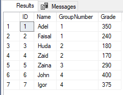
We will start with creating a new table and fill it with few records for our demo. This can be achieved using the below script:
| SQLShackDemo TABLE SetVsSelectDemo ID INT IDENTITY (1,1) PRIMARY KEY, Name NVARCHAR (50), GroupNumber INT, Grade INT INTO SetVsSelectDemo VALUES ('Adel',1,350) INTO SetVsSelectDemo VALUES ('Faisal',1,240) INTO SetVsSelectDemo VALUES ('Huda',2,180) INTO SetVsSelectDemo VALUES ('Zaid',2,170) INTO SetVsSelectDemo VALUES ('Zaina',3,290) INTO SetVsSelectDemo VALUES ('John',4,400) INTO SetVsSelectDemo VALUES ('Igor',4,375) |
The inserted data can be checked using the following SELECT statement:
| FROM SetVsSelectDemo |
And the data will be shown as below:
If we manage to assign a scalar value for the SQL variable that is previously defined using the DECLARE statement, both the SET and SELECT statements will achieve the target in the same way. The below SET statement is used to assign the @EmpName1 variable with the scalar “Ali” value:
| @EmpName1 NVARCHAR(50) @EmpName1 = 'Ali' @EmpName1 |
In the same way, the below SELECT statement can be used to assign the @EmpName2 variable with the scalar “Ali” value:
| @EmpName2 NVARCHAR(50) @EmpName2 = 'Ali' @EmpName2 |
The assigned values for the variables in the previous queries will be printed in the Messages tab as shown below:

SQL Server allows us to assign value for a SQL variable from a database table or view. The below query is used to assign the @EmpName variable the Name column value of the third group members from the SetVsSelectDemo table using the SET statement:
| @EmpName NVARCHAR(50) @EmpName = (SELECT [Name] FROM SetVsSelectDemo WHERE GroupNumber = 3) @EmpName |
The SELECT statement can be also used to perform the same assignment task in a different way as shown below:
| @EmpName NVARCHAR(50) @EmpName = [Name] FROM SetVsSelectDemo WHERE GroupNumber = 3 @EmpName |
The results of the previous two queries will be displayed in the Messages tab as shown below:

Until this point, you can see that both the SET and SELECT statements can perform the variable value assignment task in the same way and differ from the code side only.
Multiple SQL Variables
Assume that we need to assign values to multiple variables at one shot. The SET statement can assign value to one variable at a time; this means that, if we need to assign values for two variables, we need to write two SET statements. In the below example, each variable requires a separate SET statement to assign it scalar value, before printing it:
| @EmpName1 NVARCHAR(50) , @EmpName2 NVARCHAR(50) @EmpName1 = 'Ali' @EmpName2 = 'Fadi' @EmpName1 @EmpName2 |
On the other hand, the SELECT statement can be used to assign values to the previously defined multiple SQL variables using one SELECT statement. The below SELECT statement can be easily used to assign scalar values to the two variables using one SELECT statement before printing it:
| @EmpName1 NVARCHAR(50) , @EmpName2 NVARCHAR(50) @EmpName1 = 'Ali', @EmpName2 = 'Fadi' @EmpName1 @EmpName2 |
You can see from the printed result below, that both statements achieve the same task, with the SELECT statement better than the SET statement when trying to assign values to multiple variables due to code simplicity:

Again, if we try to assign values from database table to multiple variables, it requires us SET statements equal to the number of variables. In our example, we need two SET statements to assign values from the SetVsSelectDemo table to the @EmpName and @EmpGrade variables as shown in the script below:
| @EmpName NVARCHAR(50), @EmpGrade INT @EmpName = (SELECT [Name] FROM SetVsSelectDemo WHERE GroupNumber = 3) @EmpGrade = (SELECT [Grade] FROM SetVsSelectDemo WHERE GroupNumber = 3) @EmpName @EmpGrade |
On the other hand, only one SELECT statement can be used to assign values from the SetVsSelectDemo table to the @EmpName and @EmpGrade SQL variables, using simpler query as shown clearly below:
| @EmpName NVARCHAR(50), @EmpGrade INT @EmpName=[Name] , @EmpGrade =[Grade] FROM SetVsSelectDemo WHERE GroupNumber = 3 @EmpName @EmpGrade |
It is obvious from the previous two queries that the query that is using the SELECT statement is more efficient than the one using the SET statement when assigning values to multiple variables at the same time, due to the fact that, the SET statement can only assign one variable at a time. The similar results of the previous two queries that are printed in the Messages tab will be like the below in our case:

Multiple values
The second point, in which the difference between assigning values to the SQL variables using the SELECT or SET statements appears, is when the result set of the subquery query that is used to assign a value to the variable returns more than one value. In this case, the SET statement will return an error as it accepts only one scalar value from the subquery to assign it to the variable, while the SELECT statement accepts that situation, in which the subquery will return multiple values, without raising any error. You will not, though, have any control on which value will be assigned to the variable, where the last value returned from the subquery will be assigned to the variable.
Assume that we need to assign the Name value of the second group from the previously created SetVsSelectDemo table to the @EmpName SQL variable. Recall that the second group on that table contains two records in the result set as shown below:

The script that is used to assign the @EmpName variable value from the SetVsSelectDemo table using the SET and SELECT statements will be like:
| @EmpName NVARCHAR(50) @EmpName = (SELECT [Name] FROM SetVsSelectDemo WHERE GroupNumber = 2) @EmpName @EmpName NVARCHAR(50) @EmpName = [Name] FROM SetVsSelectDemo WHERE GroupNumber = 2 @EmpName |
Due to the fact that, the subquery statement returned two records, assigning value to the @EmpName SQL variable using the SET statement will fail, as the SET statement can assign only single value to the variables. This is not the case when assigning value to the @EmpName variable using the SELECT statement that will succeed with no error, assigning the name from the second returned record, which is “Zaid”, to the variable as shown in the result messages below:

We can learn from the previous result that, when you expect that the subquery will return more than one value, it is better to use the SET statement to assign value to the variable by implementing a proper error handling mechanism, rather than using the SELECT statement that will assign the last returned value to the SQL variable, with no error returned to warn us that the subquery returned multiple values.
Assign no value
Another difference between assigning values to the SQL variables using the SET and SELECT statements, is when the subquery that is used to assign a value to the variable return no value. If the previously declared variable has no initial value, both the SET and SELECT statement will act in the same way, assigning NULL value to that variable.
Assume that we need to assign the @EmpName variable, with no initial value, the Name of the fifth group from the SetVsSelectDemo table. Recall that this table has no records that belong to the fifth group as shown below:

The script that is used to assign the value to the @EmpName variable from the SetVsSelectDemo table will be like:
| @EmpName NVARCHAR(50) @EmpName = (SELECT [Name] FROM SetVsSelectDemo WHERE GroupNumber = 5) @EmpName AS SET_Name @EmpName NVARCHAR(50) @EmpName = [Name] FROM SetVsSelectDemo WHERE GroupNumber = 5 @EmpName AS SELECT_Name |
Having no initial value for the @EmpName variable, and no value returned from the subquery, a NULL value will be assigned to that variable in both cases as shown clearly in the result message below:

If the previously declared SQL variable has an initial value, and the subquery that is used to assign a value to the variable returns no value, the SET and SELECT statement will behave in different ways. In this case, the SET statement will override the initial value of the variable and return the NULL value. On the contrary, the SELECT statement will not override the initial value of the variable and will return it, if no value is returned from the assigning subquery.
If we arrange again to assign the @EmpName variable, the Name of the fifth group from the SetVsSelectDemo table, recalling that this table has no records that belong to the fifth group, but this time, after setting an initial value for the @EmpName SQL variable during the variable declaration, using the SET and SELECT statements, as shown in the script below:
| @EmpName NVARCHAR(50)='Sanya' @EmpName = (SELECT [Name] FROM SetVsSelectDemo WHERE GroupNumber = 5) @EmpName AS SET_Name @EmpName NVARCHAR(50)='Sanya' @EmpName = [Name] FROM SetVsSelectDemo WHERE GroupNumber = 5 @EmpName AS SELECT_Name |
Taking into consideration that the assigning subquery retuned no value, the query that used the SET statement to assign value to the SQL variable will override the initial value of the variable, returning NULL value, while the query that used the SELECT statement to assign value to the variable will keep the initial value with no change as no value is returned from the subquery, as shown clearly in the results below:

- If you manage to assign values to multiple variables directly or from a database table, it is better to use the SELECT statement, that requires one statement only, over the SET statement due to coding simplicity
- If you are following the ANSI standard for code migration purposes, use the SET statement for SQL variables values assignment, as the SELECT statement does not follow the ANSI standard
- If the assigning subquery returns multiple values, using the SET statement to assign value to a variable will raise an error as it only accepts a single value, where the SELECT statement will assign the last returned value from the subquery to the variable, with no control from your side
- If the assigning subquery returns no value, the SET statement will override the variable initial value to NULL, while the SELECT statement will not override its initial value
- Recent Posts

- Azure Data Factory Interview Questions and Answers - February 11, 2021
- How to monitor Azure Data Factory - January 15, 2021
- Using Source Control in Azure Data Factory - January 12, 2021
Related posts:
- Qué elegir al asignar valores a las variables de SQL Server: sentencias SET vs SELECT T-SQL
- Static Data Masking in SSMS 18
- SQL Server PRINT and SQL Server RAISERROR statements
- What is causing database slowdowns?
- SQL Variables: Basics and usage
SQL Tutorial
Sql database, sql references, sql examples, sql exercises.
You can test your SQL skills with W3Schools' Exercises.
We have gathered a variety of SQL exercises (with answers) for each SQL Chapter.
Try to solve an exercise by filling in the missing parts of a code. If you're stuck, hit the "Show Answer" button to see what you've done wrong.
Count Your Score
You will get 1 point for each correct answer. Your score and total score will always be displayed.
Start SQL Exercises
Start SQL Exercises ❯
If you don't know SQL, we suggest that you read our SQL Tutorial from scratch.
Kickstart your career
Get certified by completing the course

COLOR PICKER

Contact Sales
If you want to use W3Schools services as an educational institution, team or enterprise, send us an e-mail: [email protected]
Report Error
If you want to report an error, or if you want to make a suggestion, send us an e-mail: [email protected]
Top Tutorials
Top references, top examples, get certified.
Advanced SQL Practice: 10 Exercises with Solutions

- sql practice
Table of Contents
Practicing Your Way to SQL Proficiency
Exercise 1: list all clothing items, exercise 2: get all non-buying customers, exercise 3: select all main categories and their subcategories, exercise 4: organize runners into groups, exercise 5: how many runners participate in each event, exercise 6: group runners by main distance and age, exercise 7: list the top 3 most expensive orders, exercise 8: compute deltas between consecutive orders, exercise 9: compute the running total of purchases per customer, exercise 10: find the invitation path for each student, advancing one query at a time.
As SQL proficiency continues to be in high demand for data professionals and developers alike, the importance of hands-on practice cannot be emphasized enough. Read on to delve into the world of advanced SQL and engage in practical exercises to enhance your skills.
This article provides you with a collection of ten challenging SQL practice exercises specifically for those seeking to enhance their advanced SQL skills. The exercises cover a selection of SQL concepts and will help you refresh your advanced SQL knowledge. Each exercise is accompanied by a detailed solution, allowing you to test your knowledge and gain a deeper understanding of complex SQL concepts. The exercises come from our advanced SQL practice courses . If you want to see more exercises like this, check out these courses:
- Window Functions Practice Set
- 2021 Monthly SQL Practice Sets - Advanced
- 2022 Monthly SQL Practice Sets - Advanced
Find out how you can practice advanced SQL with our platform.
Let’s get started.
Practice is an integral component in mastering SQL; its importance cannot be overstated. The journey to becoming proficient in advanced SQL requires dedication, perseverance, and a strong commitment to continuous practice. By engaging in regular advanced SQL practice, individuals can sharpen their skills, expand their knowledge, and develop a deep understanding of the intricacies of data management and manipulation.
Advanced SQL exercises serve as invaluable tools, challenging learners to apply their theoretical knowledge in practical scenarios and further solidifying their understanding of complex concepts. With each session of dedicated SQL practice, you can discover efficient techniques and gain the confidence needed to tackle real-world data challenges.
Let’s go over the exercises and their solutions.
Advanced SQL Practice Exercises
We’ll present various advanced SQL exercises that cover window functions , JOINs, GROUP BY, common table expressions (CTEs), and more.
Section 1: Advanced SQL JOIN Exercises
In the following advanced SQL exercises, we’ll use a sportswear database that stores information about clothes, clothing categories, colors, customers, and orders. It contains five tables: color , customer , category , clothing , and clothing_order . Let's look at the data in this database.
The color table contains the following columns:
- id stores the unique ID for each color.
- name stores the name of the color.
- extra_fee stores the extra charge (if any) added for clothing ordered in this color.
In the customer table, you'll find the following columns:
- id stores customer IDs.
- first_name stores the customer's first name.
- last_name stores the customer's last name.
- favorite_color_id stores the ID of the customer's favorite color (references the color table).
The category table contains these columns:
- id stores the unique ID for each category.
- name stores the name of the category.
- parent_id stores the ID of the main category for this category (if it's a subcategory). If this value is NULL , it denotes that this category is a main category. Note: Values are related to those in the id column in this table.
The clothing table stores data in the following columns:
- id stores the unique ID for each item.
- name stores the name of that item.
- size stores the size of that clothing: S, M, L, XL, 2XL, or 3XL.
- price stores the item's price.
- color_id stores the item's color (references the color table).
- category_id stores the item's category (references the category table).
The clothing_order table contains the following columns:
- id stores the unique order ID.
- customer_id stores the ID of the customer ordering the clothes (references the customer table).
- clothing_id stores the ID of the item ordered (references the clothing table).
- items stores how many of that clothing item the customer ordered.
- order_date stores the date of the order.
Let’s do some advanced SQL exercises that focus on JOINs .
Display the name of clothing items (name the column clothes ), their color (name the column color ), and the last name and first name of the customer(s) who bought this apparel in their favorite color. Sort rows according to color, in ascending order.
Solution explanation:
We want to display the column values from three different tables ( clothing , color , and customer ), including information on which customer ordered a certain item (from the clothing_order table). Therefore, we need to join these four tables on their common columns.
First, we select from the clothing_order table (aliased as co ) and join it with the clothing table (aliased as cl ). We join the tables using the primary key column of the clothing table ( id ) and the foreign key column of the clothing_order table ( clothing_id ); this foreign key column links the clothing and clothing_order tables.
Next, we join the color table (aliased as col ) with the clothing table (aliased as cl ). Here we use the primary key column of the color table ( id ) and the foreign key column of the clothing table ( color_id ).
Finally, we join the customer table (aliased as cus ) with the clothing_order table (aliased as co ). The foreign key of the clothing_order table ( customer_id ) links to the primary key of the customer table ( id ).
The ON clause stores the condition for the JOIN statement. For example, an item from the clothing table with an id of 23 is joined with an order from the clothing_order table where the clothing_id value equals 23.
Follow this article to see more examples on JOINing three (or more) tables . And here is how to LEFT JOIN multiple tables .
Select the last name and first name of customers and the name of their favorite color for customers with no purchases.
Here we need to display customers’ first and last names from the customer table and their favorite color name from the color table. We must do it only for customers who haven’t placed any orders yet; therefore, we require information from the clothing_order table. So the next step is to join these three tables.
First, we join the customer table (aliased as cus ) with the color table (aliased as col ). To do that, we use the following condition: the primary key column of the color table ( id ) must be equal to the foreign key column of the customer table ( favorite_color_id ). That lets us select the favorite color name instead of its ID.
Here is how to ensure that we list only customers who haven’t placed any orders yet:
- We LEFT JOIN the clothing_order table (aliased as o ) with the customer table (aliased as cus ) to ensure that all rows from the customer table (even the ones with no match) are listed.
- In the WHERE clause, we define a condition to display only the rows with the customer_id column from the clothing_order table equal to NULL (meaning only the customers whose IDs are not in the clothing_order table will be returned).
There are different types of JOINs , including INNER JOIN , LEFT JOIN , RIGHT JOIN , and FULL JOIN . You can learn more by following the linked articles.
Select the name of the main categories (which have a NULL in the parent_id column) and the name of their direct subcategory (if one exists). Name the first column category and the second column subcategory.
Each category listed in the category table has its own ID (stored in the id column); some also have the ID of their parent category (stored in the parent_id column). Thus, we can link the category table with itself to list main categories and their subcategories.
The kind of JOIN where we join a table to itself is colloquially called a self join . When you join a table to itself, you must give different alias names to each copy of the table. Here we have one category table aliased as c1 and another category table aliased as c2 .
We select the name from the category table (aliased as c1 ) and ensure that we list only main categories by having its parent_id column equal to NULL in the WHERE clause. Next, we join the category table (aliased as c1 ) with the category table (aliased as c2 ). The latter one provides subcategories for the main categories. Therefore, in the ON clause, we define that the parent_id column of c2 must be equal to the id column of c1 .
Read this article to learn more about self joins .
The exercises in this section have been taken from our course 2021 Monthly SQL Practice Sets - Advanced . Every month we publish a new SQL practice course in our Monthly SQL Practice track; every odd-numbered month, the course is at an advanced level. The advanced SQL practice courses from 2021 have been collected in our 2021 Monthly SQL Practice Sets - Advanced course. Check it out to find more JOIN exercises and other advanced SQL challenges.
Section 2: Advanced GROUP BY Exercises
In the following advanced SQL exercises, we’ll use a sportsclub database that stores information about runners and running events. It contains three tables: runner , event , and runner_event . Let's look at the data in this database.
The runner table contains the following columns:
- id stores the unique ID of the runner.
- name stores the runner's name.
- main_distance stores the distance (in meters) that the runner runs during events.
- age stores the runner's age.
- is_female indicates if the runner is male or female.
The event table contains the following columns:
- id stores the unique ID of the event.
- name stores the name of the event (e.g. London Marathon, Warsaw Runs, or New Year Run).
- start_date stores the date of the event.
- city stores the city where the event takes place.
The runner_event table contains the following columns:
- runner_id stores the ID of the runner.
- event_id stores the ID of the event.
Let’s do some advanced SQL exercises that focus on GROUP BY .
Select the main distance and the number of runners that run the given distance ( runners_number ). Display only those rows where the number of runners is greater than 3.
Solution explanation :
We want to get the count of runners for each distance that they run. To do that, we need to group all runners by distance and use the COUNT() aggregate function to calculate how many runners are in each distance group.
We select the main_distance column and GROUP BY this column. Now when we use the COUNT() aggregate functions, it is going to give us the number of runners that match each main_distance value.
The GROUP BY clause is used to group rows from a table based on one or more columns. It divides the result set into subsets or groups, where each group shares the same values in the specified column(s). This allows us to perform aggregate functions (such as SUM() , COUNT() , AVG() , etc.) on each group separately.
Here are the most common GROUP BY interview questions .
To display only the groups with more than three runners, we use a HAVING clause that filters the values returned by the COUNT() aggregate function.
The HAVING clause is often used together with the GROUP BY clause to filter the grouped data based on specific conditions. It works similarly to the WHERE clause, but it operates on the grouped data rather than individual rows. Check out this article to learn more about the HAVING clause .
Display the event name and the number of club members that take part in this event (call this column runner_count ). Note that there may be events in which no club members participate. For these events, the runner_count should equal 0.
Here we want to display the event name from the event table and the number of participants from the runner table. The event and runner tables are linked by a many-to-many relation; to join these tables, we also need the runner_event table that relates events and runners.
First, we select from the event table. Then, we LEFT JOIN it with the runner_event table, which is further LEFT JOINed with the runner table. Why do we use the LEFT JOIN here? Because we want to ensure that all events (even the ones with no participants) are displayed.
We select the event name and the count of all participants; therefore, we need to GROUP BY the event name to get the count of participants per event. Please note that we use COUNT(runner_id) instead of COUNT(*) . This is to ensure that we display zero for events with no participants (i.e. for events that do not link to any runner_id ). You can read more about different variants of the COUNT() function here .
Display the distance and the number of runners there are for the following age categories: under 20, 20–29, 30–39, 40–49, and over 50. Use the following column aliases: under_20 , age_20_29 , age_30_39 , age_40_49 , and over_50 .
This is similar to Exercise 4 – we want to know the number of runners per distance value. So we select the main_distance column and GROUP BY this column. Then, we use several COUNT() aggregate functions to get the number of runners per distance. However, here we need to further divide the runners according to their age.
The CASE WHEN statement comes in handy here, as it can be used to evaluate conditions and return different values based on the results of those conditions. We can pass it as an argument to the COUNT() aggregate function to get the number of runners fulfilling a given condition. Let’s see how that works.
This CASE WHEN statement returns id only when a runner’s age is greater than or equal to 20 and less than 30. Otherwise, it returns NULL . When wrapped in the COUNT() aggregate function, it returns the count of runners fulfilling the condition defined in the CASE WHEN statement.
To get the number of runners for each of the five age groups, we need to use as many COUNT() functions and CASE WHEN statements as we have age groups. You can read about counting rows by combining CASE WHEN and GROUP BY here .
Section 3: Advanced Window Functions Exercises
In the following advanced SQL exercises, we’ll use a Northwind database for an online shop with numerous foods. It contains six tables: customers , orders , products , categories , order_items , and channels . Let's look at the data in this database.
The customers table has 15 columns:
- customer_id stores the ID of the customer.
- email stores the customer’s email address.
- full_name stores the customer’s full name.
- address stores the customer’s street and house number.
- city stores the city where the customer lives.
- region stores the customer’s region (not always applicable).
- postal_code stores the customer’s ZIP/post code.
- country stores the customer’s country.
- phone stores the customer’s phone number.
- registration_date stores the date on which the customer registered.
- channel_id stores the ID of the channel through which the customer found the shop.
- first_order_id stores the ID of the first order made by the customer.
- first_order_date stores the date of the customer’s first order.
- last_order_id stores the ID of the customer’s last (i.e. most recent) order.
- last_order_date stores the date of the customer’s last order.
The orders table has the following columns:
- order_id stores the ID of the order.
- customer_id stores the ID of the customer who placed the order.
- order_date stores the date when the order was placed.
- total_amount stores the total amount paid for the order.
- ship_name stores the name of the person to whom the order was sent.
- ship_address stores the address (house number and street) where the order was sent.
- ship_city stores the city where the order was sent.
- ship_region stores the region in which the city is located.
- ship_postalcode stores the destination post code.
- ship_country stores the destination country.
- shipped_date stores the date when the order was shipped.
The products table has the following columns:
- product_id stores the ID of the product.
- product_name stores the name of the product.
- category_id stores the category to which the product belongs.
- unit_price stores the price for one unit of the product (e.g. per bottle, pack, etc.).
- discontinued indicates if the product is no longer sold.
The categories table has the following columns:
- category_id stores the ID of the category.
- category_name stores the name of the category.
- description stores a short description of the category.
The order_items table has the following columns:
- order_id stores the ID of the order in which the product was bought.
- product_id stores the ID of the product purchased in the order.
- unit_price stores the per-unit price of the product. (Note that this can be different from the price in the product’s category; the price can change over time and discounts can be applied.)
- quantity stores the number of units bought in the order.
- discount stores the discount applied to the given product.
The channels table has the following columns:
- channel_name stores the name of the channel through which the customer found the shop.
Let’s do some advanced SQL exercises that focus on window functions.
Create a dense ranking of the orders based on their total_amount . The bigger the amount, the higher the order should be. If two orders have the same total_amount , the older order should go higher (you'll have to add the column order_date to the ordering). Name the ranking column rank . After that, select only the orders with the three highest dense rankings . Show the rank, order_id , and total_amount .
Let’s start with the first part of the instruction. We want to create a dense ranking of orders based on their total_amount (the greater the value, the higher the rank) and their order_date value (the older the date, the higher the rank). Please note that the rank value may be duplicated only when total_amount and order_date columns are both equal for more than one row.
To do that, we use the DENSE_RANK() window function. In its OVER() clause, we specify the order: descending for total_amount values and ascending for order_date values. We also display the order_id and total_amount columns from the orders table.
Until now, we listed all orders along with their dense rank values. But we want to see only the top 3 orders (where the rank column is less than or equal to 3). Let’s analyze the steps we take from here:
- We define a Common Table Expression (CTE) using this SELECT statement – i.e. we use the WITH clause followed by the CTE’s name and then place the SELECT statement within parentheses.
- Then we select from this CTE, providing the condition for the rank column in the WHERE clause.
You may wonder why we need such a complex syntax that defines a CTE and then queries it. You may say that we could set the condition for the rank column in the WHERE clause of the first SELECT query. Well, that’s not possible because of the SQL query order of execution.
We have to use the Common Table Expression here because you can’t use window functions in the WHERE clause. The order of operations in SQL is as follows:
- FROM , JOIN
- Aggregate functions
- Window functions
You may only use window functions in SELECT and ORDER BY clauses. If you want to refer to window functions in the WHERE clause, you must place the window function computation in a CTE (like we did in our example) or in a subquery and refer to the window function in the outer query.
Follow this article to learn more about CTEs and recursive CTEs .
To give you some background on the available ranking functions , there are three functions that let you rank your data: RANK() , DENSE_RANK() , and ROW_NUMBER() . Let’s see them in action.
| Values to be ranked | RANK() | DENSE_RANK() | ROW_NUMBER() |
|---|---|---|---|
| 1 | 1 | 1 | 1 |
| 1 | 1 | 1 | 2 |
| 1 | 1 | 1 | 3 |
| 2 | 4 | 2 | 4 |
| 3 | 5 | 3 | 5 |
| 3 | 5 | 3 | 6 |
| 4 | 7 | 4 | 7 |
| 5 | 8 | 5 | 8 |
The RANK() function assigns the same rank if multiple consecutive rows have the same value. Then, the next row gets the next rank as if the previous rows had distinct values. Here, the ranks 1,1,1 are followed by 4 (as if it was 1,2,3 instead of 1,1,1 ).
The DENSE_RANK() function also assigns the same rank if multiple consecutive rows have the same value. Then, the next row gets the next rank one greater than the previous one. Here, 1,1,1 is followed by 2.
The ROW_NUMBER() function assigns consecutive numbers to each next row without considering the row values.
Here is an article on how to rank data . You can also learn more about differences between SQL’s ranking functions .
In this exercise, we're going to compute the difference between two consecutive orders from the same customer.
Show the ID of the order ( order_id ), the ID of the customer ( customer_id ), the total_amount of the order, the total_amount of the previous order based on the order_date (name the column previous_value ), and the difference between the total_amount of the current order and the previous order (name the column delta ).
Here we select the order ID, customer ID, and total amount from the orders table. The LAG() function fetches the previous total_amount value. In the OVER() clause, we define the LAG() function separately for each customer and order the outcome by an order date. Finally, we subtract the value returned by the LAG() function from the total_amount value for each row to get the delta.
The previous_value column stores null for the first row, as there are no previous values. Therefore, the delta column is also null for the first row. The following delta column values store the differences between consecutive orders made by the same customer.
It is worth mentioning that a delta represents the difference between two values. By calculating the delta between daily sales amounts, we can determine the direction of sales growth/decline on a day-to-day basis.
Follow this article to learn more about calculating differences between two rows . And here is how to compute year-over-year differences .
For each customer and their orders, show the following:
- customer_id – the ID of the customer.
- full_name – the full name of the customer.
- order_id – the ID of the order.
- order_date – the date of the order.
- total_amount – the total spent on this order.
- running_total – the running total spent by the given customer.
Sort the rows by customer ID and order date.
A running total refers to the calculation that accumulates the values of a specific column or expression as rows are processed in a result set. It provides a running sum of the values encountered up to the current row. A running total is calculated by adding the current value to the sum of all previous values. This can be particularly useful in various scenarios, such as tracking cumulative sales, calculating running balances or analyzing cumulative progress over time.
Follow this article to learn more about computing a running total . And here is an article about computing running averages .
We select customer ID, order ID, order date, and order total from the orders table. Then, we join the orders table with the customers table on their respective customer_id columns so we can display the customer's full name.
We use the SUM() window function to calculate the running total for each customer separately ( PARTITION BY orders.customer_id ) and then order ascendingly by date ( ORDER BY orders.order_date ).
Finally, we order the output of this query by customer ID and order date.
Section 4: Advanced Recursive Query Exercises
In the following advanced SQL exercises, we’ll use a website database that stores information about students and courses. It contains three tables: student , course , and student_course . Let's look at the data in this database.
The student table contains the following columns:
- id stores the unique ID number for each student.
- name stores the student's name.
- email stores the student's email.
- invited_by_id stores the ID of the student that invited this student to the website. If the student signed up without an invitation, this column will be NULL.
The course table consists of the following columns:
- id stores the unique ID number for each course.
- name stores the course's name.
The student_course table contains the following columns:
- id stores the unique ID for each row.
- student_id stores the ID of the student.
- course_id stores the ID of the course.
- minutes_spent stores the number of minutes the student spent on the course.
- is_completed is set to True when the student finishes the course.
The exercises in this section have been taken from our Window Functions Practice Set . In this set, you will find more window function exercises on databases that store retail, track competitions, and website traffic.
Let’s do some advanced SQL exercises that focus on recursive queries.
Show the path of invitations for each student (name this column path ). For example, if Mary was invited by Alice and Alice wasn't invited by anyone, the path for Mary should look like this: Alice->Mary .
Include each student's id , name , and invited_by_id in the results.
This exercise requires us to create a custom value for the path column that contains the invitation path for each customer. For example, Ann Smith was invited by Veronica Knight , who in turn was invited by Karli Roberson ; hence, we get the path column as Karli Roberson->Veronica Knight->Ann Smith for the name Ann Smith .
As you may notice, we need a recursion mechanism to dig down into the invitation path. We can write a recursive query by defining it with the WITH RECURSIVE statement, followed by the query name.
The content of the hierarchy recursive query is as follows:
- We select the id , name , and invited_by_id columns from the student table. Then, we use the CAST() function to cast the name column type to the TEXT data type, ensuring smooth concatenation (with -> and the following names) in the main query. The WHERE clause condition ensures that only students who haven’t been invited are listed by this query.
- The UNION ALL operator combines the result sets of two or more SELECT statements without removing duplicates. Here the queries on which UNION ALL is performed have the same sets of four columns; the result set of one is appended to the results set of another.
- In the next SELECT statement, we again select the id , name , and invited_by_id columns from the student table. Then, we concatenate the path column (that comes from the hierarchy recursive query as defined in the first SELECT statement) with the -> sign and the student name. To accomplish this concatenation, we select from both the student table and the hierarchy recursive query.(This is where the recursive mechanism comes into play.) In the WHERE clause, we define that the invited_by_id column of the student table is equal to the id column of the hierarchy recursive query, so we get the student name who invited the current student; on the next iteration, we get the name of the student who invited that student, and so on.
This is called a recursive query, as it queries itself to work its way down the invitation path.
The advanced SQL exercises presented in this article provide a comprehensive platform for honing your SQL skills, one query at a time. By delving into window functions, JOINs , GROUP BY , and more, you have expanded your understanding of complex SQL concepts and gained hands-on experience in solving real-world data challenges.
Practice is the key to mastering SQL skills. Through consistent practice, you can elevate your proficiency and transform your theoretical knowledge into practical expertise. This article showcased exercises from our courses; you can discover more exercises like this by enrolling in our:
Sign up now and get started for free! Good luck!
You may also like

How Do You Write a SELECT Statement in SQL?

What Is a Foreign Key in SQL?

Enumerate and Explain All the Basic Elements of an SQL Query
- SQL Cheat Sheet
- SQL Interview Questions
- MySQL Interview Questions
- PL/SQL Interview Questions
- Learn SQL and Database
SQL Exercises : SQL Practice with Solution for Beginners and Experienced
SQL ( Structured Query Language ) is a powerful tool used for managing and manipulating relational databases. Whether we are beginners or experienced professionals, practicing SQL exercises is important for improving your skills. Regular practice helps you get better at using SQL and boosts your confidence in handling different database tasks.
So, in this free SQL exercises page, we’ll cover a series of SQL practice exercises covering a wide range of topics suitable for beginners , intermediate , and advanced SQL learners. These exercises are designed to provide hands-on experience with common SQL tasks, from basic retrieval and filtering to more advanced concepts like joins window functions , and stored procedures.
Table of Content
SQL Exercises for Practice
Sql practice exercises for beginners, sql practice exercises for intermediate, sql practice exercises for advanced, more questions for practice.
Practice SQL questions to enhance our skills in database querying and manipulation. Each question covers a different aspect of SQL , providing a comprehensive learning experience.

We have covered a wide range of topics in the sections beginner , intermediate and advanced .
- Basic Retrieval
- Arithmetic Operations and Comparisons:
- Aggregation Functions
- Group By and Having
- Window Functions
- Conditional Statements
- DateTime Operations
- Creating and Aliasing
- Constraints
- Stored Procedures:
- Transactions
let’s create the table schemas and insert some sample data into them.
Create Sales table
| sale_id | product_id | quantity_sold | sale_date | total_price |
|---|---|---|---|---|
| 1 | 101 | 5 | 2024-01-01 | 2500.00 |
| 2 | 102 | 3 | 2024-01-02 | 900.00 |
| 3 | 103 | 2 | 2024-01-02 | 60.00 |
| 4 | 104 | 4 | 2024-01-03 | 80.00 |
| 5 | 105 | 6 | 2024-01-03 | 90.00 |
Create Products table
| product_id | product_name | category | unit_price |
|---|---|---|---|
| 101 | Laptop | Electronics | 500.00 |
| 102 | Smartphone | Electronics | 300.00 |
| 103 | Headphones | Electronics | 30.00 |
| 104 | Keyboard | Electronics | 20.00 |
| 105 | Mouse | Electronics | 15.00 |
This hands-on approach provides a practical environment for beginners to experiment with various SQL commands, gaining confidence through real-world scenarios. By working through these exercises, newcomers can solidify their understanding of fundamental concepts like data retrieval, filtering, and manipulation, laying a strong foundation for their SQL journey.
1. Retrieve all columns from the Sales table.
Explanation:
This SQL query selects all columns from the Sales table, denoted by the asterisk (*) wildcard. It retrieves every row and all associated columns from the Sales table.
2. Retrieve the product_name and unit_price from the Products table.
| product_name | unit_price |
|---|---|
| Laptop | 500.00 |
| Smartphone | 300.00 |
| Headphones | 30.00 |
| Keyboard | 20.00 |
| Mouse | 15.00 |
This SQL query selects the product_name and unit_price columns from the Products table. It retrieves every row but only the specified columns, which are product_name and unit_price.
3. Retrieve the sale_id and sale_date from the Sales table.
| sale_id | sale_date |
|---|---|
| 1 | 2024-01-01 |
| 2 | 2024-01-02 |
| 3 | 2024-01-02 |
| 4 | 2024-01-03 |
| 5 | 2024-01-03 |
This SQL query selects the sale_id and sale_date columns from the Sales table. It retrieves every row but only the specified columns, which are sale_id and sale_date.
4. Filter the Sales table to show only sales with a total_price greater than $100.
| sale_id | product_id | quantity_sold | sale_date | total_price |
|---|---|---|---|---|
| 1 | 101 | 5 | 2024-01-01 | 2500.00 |
| 2 | 102 | 3 | 2024-01-02 | 900.00 |
This SQL query selects all columns from the Sales table but only returns rows where the total_price column is greater than 100. It filters out sales with a total_price less than or equal to $100.
5. Filter the Products table to show only products in the ‘Electronics’ category.
This SQL query selects all columns from the Products table but only returns rows where the category column equals ‘Electronics’. It filters out products that do not belong to the ‘Electronics’ category.
6. Retrieve the sale_id and total_price from the Sales table for sales made on January 3, 2024.
| sale_id | total_price |
|---|---|
| 4 | 80.00 |
| 5 | 90.00 |
This SQL query selects the sale_id and total_price columns from the Sales table but only returns rows where the sale_date is equal to ‘2024-01-03’. It filters out sales made on any other date.
7. Retrieve the product_id and product_name from the Products table for products with a unit_price greater than $100.
| product_id | product_name |
|---|---|
| 101 | Laptop |
| 102 | Smartphone |
This SQL query selects the product_id and product_name columns from the Products table but only returns rows where the unit_price is greater than $100. It filters out products with a unit_price less than or equal to $100.
8. Calculate the total revenue generated from all sales in the Sales table.
| total_revenue |
|---|
| 3630.00 |
This SQL query calculates the total revenue generated from all sales by summing up the total_price column in the Sales table using the SUM() function.
9. Calculate the average unit_price of products in the Products table.
| average_unit_price |
|---|
| 173 |
This SQL query calculates the average unit_price of products by averaging the values in the unit_price column in the Products table using the AVG() function.
10. Calculate the total quantity_sold from the Sales table.
| total_quantity_sold |
|---|
| 20 |
This SQL query calculates the total quantity_sold by summing up the quantity_sold column in the Sales table using the SUM() function.
11. Retrieve the sale_id, product_id, and total_price from the Sales table for sales with a quantity_sold greater than 4.
| sale_id | product_id | total_price |
|---|---|---|
| 1 | 101 | 2500.00 |
| 5 | 105 | 90.00 |
This SQL query selects the sale_id, product_id, and total_price columns from the Sales table but only returns rows where the quantity_sold is greater than 4.
12. Retrieve the product_name and unit_price from the Products table, ordering the results by unit_price in descending order.
This SQL query selects the product_name and unit_price columns from the Products table and orders the results by unit_price in descending order using the ORDER BY clause with the DESC keyword.
13. Retrieve the total_price of all sales, rounding the values to two decimal places.
| product_name |
|---|
| 3630.00 |
This SQL query calculates the total sales revenu by summing up the total_price column in the Sales table and rounds the result to two decimal places using the ROUND() function.
14. Calculate the average total_price of sales in the Sales table.
| average_total_price |
|---|
| 726.000000 |
This SQL query calculates the average total_price of sales by averaging the values in the total_price column in the Sales table using the AVG() function.
15. Retrieve the sale_id and sale_date from the Sales table, formatting the sale_date as ‘YYYY-MM-DD’.
| sale_id | formatted_date |
|---|---|
| 1 | 2024-01-01 |
| 2 | 2024-01-02 |
| 3 | 2024-01-02 |
| 4 | 2024-01-03 |
| 5 | 2024-01-03 |
This SQL query selects the sale_id and sale_date columns from the Sales table and formats the sale_date using the DATE_FORMAT() function to display it in ‘YYYY-MM-DD’ format.
16. Calculate the total revenue generated from sales of products in the ‘Electronics’ category.
This SQL query calculates the total revenue generated from sales of products in the ‘Electronics’ category by joining the Sales table with the Products table on the product_id column and filtering sales for products in the ‘Electronics’ category.
17. Retrieve the product_name and unit_price from the Products table, filtering the unit_price to show only values between $20 and $600.
| product_name | unit_price |
|---|---|
| Laptop | 500.00 |
| Smartphone | 300.00 |
| Headphones | 30.00 |
| Keyboard | 20.00 |
This SQL query selects the product_name and unit_price columns from the Products table but only returns rows where the unit_price falls within the range of $50 and $200 using the BETWEEN operator.
18. Retrieve the product_name and category from the Products table, ordering the results by category in ascending order.
| product_name | category |
|---|---|
| Laptop | Electronics |
| Smartphone | Electronics |
| Headphones | Electronics |
| Keyboard | Electronics |
| Mouse | Electronics |
This SQL query selects the product_name and category columns from the Products table and orders the results by category in ascending order using the ORDER BY clause with the ASC keyword.
19. Calculate the total quantity_sold of products in the ‘Electronics’ category.
This SQL query calculates the total quantity_sold of products in the ‘Electronics’ category by joining the Sales table with the Products table on the product_id column and filtering sales for products in the ‘Electronics’ category.
20. Retrieve the product_name and total_price from the Sales table, calculating the total_price as quantity_sold multiplied by unit_price.
| product_name | total_price |
|---|---|
| Laptop | 2500.00 |
| Smartphone | 900.00 |
| Headphones | 60.00 |
| Keyboard | 80.00 |
| Mouse | 90.00 |
This SQL query retrieves the product_name from the Sales table and calculates the total_price by multiplying quantity_sold by unit_price, joining the Sales table with the Products table on the product_id column.
These exercises are designed to challenge you beyond basic queries, delving into more complex data manipulation and analysis. By tackling these problems, you’ll solidify your understanding of advanced SQL concepts like joins, subqueries, functions, and window functions, ultimately boosting your ability to work with real-world data scenarios effectively.
1. Calculate the total revenue generated from sales for each product category.
| category | total_revenue |
|---|---|
| Electronics | 3630.00 |
This query joins the Sales and Products tables on the product_id column, groups the results by product category, and calculates the total revenue for each category by summing up the total_price.
2. Find the product category with the highest average unit price.
| category |
|---|
| Electronics |
This query groups products by category, calculates the average unit price for each category, orders the results by the average unit price in descending order, and selects the top category with the highest average unit price using the LIMIT clause.
3. Identify products with total sales exceeding $500.
| product_name |
|---|
| Headphones |
| Keyboard |
| Laptop |
| Mouse |
| Smartphone |
This query joins the Sales and Products tables on the product_id column, groups the results by product name, calculates the total sales revenue for each product, and selects products with total sales exceeding 30 using the HAVING clause.
4. Count the number of sales made in each month.
| month | sales_count |
|---|---|
| 2024-01 | 5 |
This query formats the sale_date column to extract the month and year, groups the results by month, and counts the number of sales made in each month.
5. Determine the average quantity sold for products with a unit price greater than $100.
| average_quantity_sold |
|---|
| 4.0000 |
This query joins the Sales and Products tables on the product_id column, filters products with a unit price greater than $100, and calculates the average quantity sold for those products.
6. Retrieve the product name and total sales revenue for each product.
| product_name | total_revenue |
|---|---|
| Laptop | 2500.00 |
| Smartphone | 900.00 |
| Headphones | 60.00 |
| Keyboard | 80.00 |
| Mouse | 90.00 |
This query joins the Sales and Products tables on the product_id column, groups the results by product name, and calculates the total sales revenue for each product.
7. List all sales along with the corresponding product names.
| sale_id | product_name |
|---|---|
| 1 | Laptop |
| 2 | Smartphone |
| 3 | Headphones |
| 4 | Keyboard |
| 5 | Mouse |
This query joins the Sales and Products tables on the product_id column and retrieves the sale_id and product_name for each sale.
8. Retrieve the product name and total sales revenue for each product.
| category | category_revenue | revenue_percentage |
|---|---|---|
| Electronics | 3630.00 | 100.000000 |
This query will give you the top three product categories contributing to the highest percentage of total revenue generated from sales. However, if you only have one category (Electronics) as in the provided sample data, it will be the only result.
9. Rank products based on total sales revenue.
| product_name | total_revenue | revenue_rank |
|---|---|---|
| Laptop | 2500.00 | 1 |
| Smartphone | 900.00 | 2 |
| Mouse | 90.00 | 3 |
| Keyboard | 80.00 | 4 |
| Headphones | 60.00 | 5 |
This query joins the Sales and Products tables on the product_id column, groups the results by product name, calculates the total sales revenue for each product, and ranks products based on total sales revenue using the RANK () window function.
10. Calculate the running total revenue for each product category.
| category | product_name | sale_date | running_total_revenue |
|---|---|---|---|
| Electronics | Laptop | 2024-01-01 | 2500.00 |
| Electronics | Smartphone | 2024-01-02 | 3460.00 |
| Electronics | Headphones | 2024-01-02 | 3460.00 |
| Electronics | Keyboard | 2024-01-03 | 3630.00 |
| Electronics | Mouse | 2024-01-03 | 3630.00 |
This query joins the Sales and Products tables on the product_id column, partitions the results by product category, orders the results by sale date, and calculates the running total revenue for each product category using the SUM() window function.
11. Categorize sales as “High”, “Medium”, or “Low” based on total price (e.g., > $200 is High, $100-$200 is Medium, < $100 is Low).
| sale_id | sales_category |
|---|---|
| 1 | High |
| 2 | High |
| 3 | Low |
| 4 | Low |
| 5 | Low |
This query categorizes sales based on total price using a CASE statement. Sales with a total price greater than $200 are categorized as “High”, sales with a total price between $100 and $200 are categorized as “Medium”, and sales with a total price less than $100 are categorized as “Low”.
12. Identify sales where the quantity sold is greater than the average quantity sold.
| sale_id | product_id | quantity_sold | sale_date | total_price |
|---|---|---|---|---|
| 1 | 101 | 5 | 2024-01-01 | 2500.00 |
| 5 | 105 | 6 | 2024-01-03 | 90.00 |
This query selects all sales where the quantity sold is greater than the average quantity sold across all sales in the Sales table.
13. Extract the month and year from the sale date and count the number of sales for each month.
| month | sales_count |
|---|---|
| 2024-01 | 5 |
14. Calculate the number of days between the current date and the sale date for each sale.
| sale_id | days_since_sale |
|---|---|
| 1 | 185 |
| 2 | 184 |
| 3 | 184 |
| 4 | 183 |
| 5 | 183 |
This query calculates the number of days between the current date and the sale date for each sale using the DATEDIFF function.
15. Identify sales made during weekdays versus weekends.
| sale_id | day_type |
|---|---|
| 1 | Weekday |
| 2 | Weekday |
| 3 | Weekday |
| 4 | Weekend |
| 5 | Weekend |
This query categorizes sales based on the day of the week using the DAYOFWEEK function. Sales made on Sunday (1) or Saturday (7) are categorized as “Weekend”, while sales made on other days are categorized as “Weekday”.
This section likely dives deeper into complex queries, delving into advanced features like window functions, self-joins, and intricate data manipulation techniques. By tackling these challenging exercises, users can refine their SQL skills and tackle real-world data analysis scenarios with greater confidence and efficiency.
1. Write a query to create a view named Total_Sales that displays the total sales amount for each product along with their names and categories.
| product_name | category | total_sales_amount |
|---|---|---|
| Laptop | Electronics | 2500.00 |
| Smartphone | Electronics | 900.00 |
| Headphones | Electronics | 60.00 |
| Keyboard | Electronics | 80.00 |
| Mouse | Electronics | 90.00 |
This query creates a view named Total_Sales that displays the total sales amount for each product along with their names and categories.
2. Retrieve the product details (name, category, unit price) for products that have a quantity sold greater than the average quantity sold across all products.
| product_name | category | unit_price |
|---|---|---|
| Laptop | Electronics | 500.00 |
| Mouse | Electronics | 15.00 |
This query retrieves the product details (name, category, unit price) for products that have a quantity sold greater than the average quantity sold across all products.
3. Explain the significance of indexing in SQL databases and provide an example scenario where indexing could significantly improve query performance in the given schema.
| sale_id | product_id | quantity_sold | sale_date | total_price |
|---|---|---|---|---|
| 4 | 104 | 4 | 2024-01-03 | 80.00 |
| 5 | 105 | 6 | 2024-01-03 | 90.00 |
With an index on the sale_date column, the database can quickly locate the rows that match the specified date without scanning the entire table. The index allows for efficient lookup of rows based on the sale_date value, resulting in improved query performance.
4. Add a foreign key constraint to the Sales table that references the product_id column in the Products table.
This query adds a foreign key constraint to the Sales table that references the product_id column in the Products table, ensuring referential integrity between the two tables.
5. Create a view named Top_Products that lists the top 3 products based on the total quantity sold.
| product_name | total_quantity_sold |
|---|---|
| Mouse | 6 |
| Laptop | 5 |
| Keyboard | 4 |
This query creates a view named Top_Products that lists the top 3 products based on the total quantity sold.
6. Implement a transaction that deducts the quantity sold from the Products table when a sale is made in the Sales table, ensuring that both operations are either committed or rolled back together.
The quantity in stock for product with product_id 101 should be updated to 5.The transaction should be committed successfully.
7. Create a query that lists the product names along with their corresponding sales count.
| product_name | sales_count |
|---|---|
| Headphones | 1 |
| Keyboard | 1 |
| Laptop | 1 |
| Mouse | 1 |
| Smartphone | 1 |
This query selects the product names from the Products table and counts the number of sales (using the COUNT() function) for each product by joining the Sales table on the product_id. The results are grouped by product name using the GROUP BY clause.
8. Write a query to find all sales where the total price is greater than the average total price of all sales.
The subquery (SELECT AVG(total_price) FROM Sales) calculates the average total price of all sales. The main query selects all columns from the Sales table where the total price is greater than the average total price obtained from the subquery.
9. Analyze the performance implications of indexing the sale_date column in the Sales table, considering the types of queries commonly executed against this column.
Query without indexing:.
| Operation | Details |
|---|---|
| Filter: (sales.sale_date = DATE’2024-01-01′) | (cost=0.75 rows=1) (actual time=0.020..0.031 rows=1 loops=1) |
| Table scan on Sales | (cost=0.75 rows=5) (actual time=0.015..0.021 rows=5 loops=1) |
Query with Indexing:
| Operation | Details |
|---|---|
| Index lookup on Sales using idx_sale_date (sale_date=DATE’2024-01-01′) | (cost=0.35 rows=1) (actual time=0.024..0.024 rows=1 loops=1) |
This format clearly displays the operations and details of the query execution plan before and after indexing.
Without indexing, the query performs a full table scan, filtering rows based on the sale date, which is less efficient. With indexing, the query uses the index to quickly locate the relevant rows, significantly improving query performance.
10. Add a check constraint to the quantity_sold column in the Sales table to ensure that the quantity sold is always greater than zero.
| sale_id | product_id | quantity_sold | sale_date | total_price |
|---|---|---|---|---|
| 1 | 101 | 5 | 2024-01-01 | 2500.00 |
| 2 | 102 | 3 | 2024-01-02 | 900.00 |
| 3 | 103 | 2 | 2024-01-02 | 60.00 |
| 4 | 104 | 4 | 2024-01-03 | 80.00 |
| 5 | 105 | 6 | 2024-01-03 | 90.00 |
All rows in the Sales table meet the condition of the check constraint, as each quantity_sold value is greater than zero.
11. Create a view named Product_Sales_Info that displays product details along with the total number of sales made for each product.
| product_id | product_name | category | unit_price | total_sales |
|---|---|---|---|---|
| 101 | Laptop | Electronics | 500.00 | 1 |
| 102 | Smartphone | Electronics | 300.00 | 1 |
| 103 | Headphones | Electronics | 30.00 | 1 |
| 104 | Keyboard | Electronics | 20.00 | 1 |
| 105 | Mouse | Electronics | 15.00 | 1 |
This view provides a concise and organized way to view product details alongside their respective sales information, facilitating analysis and reporting tasks.
12. Develop a stored procedure named Update_Unit_Price that updates the unit price of a product in the Products table based on the provided product_id.
The above SQL code creates a stored procedure named Update_Unit_Price. This stored procedure takes two parameters: p_product_id (the product ID for which the unit price needs to be updated) and p_new_price (the new unit price to set).
13. Implement a transaction that inserts a new product into the Products table and then adds a corresponding sale record into the Sales table, ensuring that both operations are either fully completed or fully rolled back.
| product_id | product_name | category | unit_price |
|---|---|---|---|
| 101 | Laptop | Electronics | 550.00 |
| 102 | Smartphone | Electronics | 300.00 |
| 103 | Headphones | Electronics | 30.00 |
| 104 | Keyboard | Electronics | 20.00 |
| 105 | Mouse | Electronics | 15.00 |
This will update the unit price of the product with product_id 101 to 550.00 in the Products table.
14. Write a query that calculates the total revenue generated from each category of products for the year 2024.
| category | total_revenue |
|---|---|
| Electronics | 3630.00 |
When you execute this query, you will get the total revenue generated from each category of products for the year 2024.
If you’re looking to sharpen your SQL skills and gain more confidence in querying database s, consider delving into these articles. They’re packed with query-based SQL questions designed to enhance your understanding and proficiency in SQL .
By practicing with these exercises, you’ll not only improve your SQL abilities but also boost your confidence in tackling various database-related tasks. The Questions are as follows:
- How to Insert a Value that Contains an Apostrophe in SQL?
- How to Select Row With Max Value in SQL?
- How to Efficiently Convert Rows to Columns in SQL?
- How To Use Nested Select Queries in SQL
- How to Select Row With Max Value on a Column in SQL?
- How to Specify Condition in Count() in SQL?
- How to Find the Maximum of Multiple Columns in SQL?
- How to Update Top 100 Records in SQL?
- How to Select the Last Records in a One-To-Many Relationship Using SQL Join
- How to Join First Row in SQL?
- How to Insert Row If Not Exists in SQL?
- How to Use GROUP BY to Concatenate Strings in SQL?
- How Inner Join works in LINQ to SQL
- How to Get the Identity of an Inserted Row in SQL
- How to Declare a Variable in SQL?
Mastering SQL requires consistent practice and hands-on experience. By working through these SQL practice exercises , you’ll strengthen your skills and gain confidence in querying relational databases.
Whether you’re just starting or looking to refine your expertise, these exercises provide valuable opportunities to hone your SQL abilities. Keep practicing , and you’ll be well-equipped to tackle real-world data challenges with SQL.
Please Login to comment...
Similar reads, improve your coding skills with practice.
What kind of Experience do you want to share?
- ▼SQL Exercises
- Introduction
- Retrieve data from tables
- Boolean and Relational Operators
- Wildcard and Special operators
- Aggregate Functions
- Formatting query output
- Query on Multiple Tables
- FILTERING and SORTING on HR Database
- SUBQUERIES on HR Database
- JOINS on HR Database
- SQL User Management
- ▼Movie Database
- BASIC QUERIES
- ▼Soccer Database
- ▼Hospital Database
- ▼Employee Database
- ▼AdventureWorks Database
- ▼SQL Challenges
- Challenges-1
- ..More to come..
SQL Exercises, Practice, Solution
What is sql.
SQL stands for Structured Query Language and it is an ANSI standard computer language for accessing and manipulating database systems. It is used for managing data in relational database management system which stores data in the form of tables and relationship between data is also stored in the form of tables. SQL statements are used to retrieve and update data in a database.
The best way we learn anything is by practice and exercise questions. We have started this section for those (beginner to intermediate) who are familiar with SQL . Hope, these exercises help you to improve your SQL skills. Currently following sections are available, we are working hard to add more exercises. Happy Coding!
You may read our SQL tutorial before solving the following exercises.
List of SQL Exercises
- SQL Retrieve data from tables [33 Exercises]
- SQL Boolean and Relational operators [12 Exercises]
- SQL Wildcard and Special operators [22 Exercises]
- SQL Aggregate Functions [25 Exercises]
- SQL Formatting query output [10 Exercises]
- SQL Quering on Multiple Tables [8 Exercises]
- FILTERING and SORTING on HR Database [38 Exercises]
- SQL JOINS [29 Exercises]
- SQL JOINS on HR Database [27 Exercises]
- SQL SUBQUERIES
- SQL SUBQUERIES [39 Exercises]
- SQL SUBQUERIES on HR Database [55 Exercises]
- SQL Union[9 Exercises]
- SQL View[16 Exercises]
- SQL User Account Management [16 Exercise]
- Movie Database
- BASIC queries on movie Database [10 Exercises]
- SUBQUERIES on movie Database [16 Exercises]
- JOINS on movie Database [24 Exercises]
- Soccer Database
- BASIC queries on soccer Database [29 Exercises]
- SUBQUERIES on soccer Database [33 Exercises]
- JOINS queries on soccer Database [61 Exercises]
- Hospital Database
- BASIC, SUBQUERIES, and JOINS [41 Exercises]
- Employee Database
- BASIC queries on employee Database [115 Exercises]
- SUBQUERIES on employee Database [77 Exercises]
- AdventureWorks Database:
- AdventureWorks Database [200 Exercises]
- SQL Challenges-1:
- SQL Challenges-1 [77 Exercises]
- More to come!
Structure of inventory database :

Structure of HR database :
Structure of movie database :

Structure of soccer database :

Structure of employee database :

Structure of hospital database :

Syntax diagram of SQL SELECT statement

You may download the structure and data of the tables of database on which SQL Exercises are built.
Please note that PostgreSQL 9.4 is used and the file which you would download is generated using pg_dump
Follow us on Facebook and Twitter for latest update.
- Weekly Trends and Language Statistics
- Stack Overflow for Teams Where developers & technologists share private knowledge with coworkers
- Advertising & Talent Reach devs & technologists worldwide about your product, service or employer brand
- OverflowAI GenAI features for Teams
- OverflowAPI Train & fine-tune LLMs
- Labs The future of collective knowledge sharing
- About the company Visit the blog
Collectives™ on Stack Overflow
Find centralized, trusted content and collaborate around the technologies you use most.
Q&A for work
Connect and share knowledge within a single location that is structured and easy to search.
Get early access and see previews of new features.
Assign to a T-SQL variable from a CASE statement
I'd like to assign some variables inside a query that uses CASE statements for it's columns. Not quite sure how to do this, having trouble finding the right syntax.
This is what I have so far, but it's got syntax errors.
What's the correct place/way to stick those variables in there?
- Can you be more specific as to how "it's not quite working"? – Adam Robinson Commented Aug 4, 2011 at 17:37
- I'm putting my variable assignment in the wrong place and it causes a syntax error. I'm not sure where/how to put the variable assignment. – rlb.usa Commented Aug 4, 2011 at 17:39
- 3 What you have posted works well for me. Your issue may not be in the assignment, but the actual code. Can you post the actual code? – Raj More Commented Aug 4, 2011 at 17:41
3 Answers 3
The example you've given should work. You can assign to variables from a case statement. Just pretend that the entire CASE..WHEN..THEN..ELSE..END block is a field. Here is a generic example:
Can you tell us what specific error(s) you are getting?
You could probably do this more easily using ISNULL or COALESCE :
- 2 This is true in his particular case, but does not answer the question. – Adam Robinson Commented Aug 4, 2011 at 17:49
- I disagree. Getting the desired functionality working while improving the code seems like an excellent answer. Also, his original code didn't appear to be broken... – Abe Miessler Commented Aug 4, 2011 at 18:15
- I think you might be biased as to what might make an excellent answer to this question ;) If he'd asked the question in a broader way (i.e. stating his goals rather than asking questions about a particular implemention), then I'd agree with you, but he asked about assigning values to variables using a case statement, which is a perfectly valid use case that, in this particular case can be replaced with a different solution. Recommending alternatives is certainly good, but the original question needs to be addressed first. – Adam Robinson Commented Aug 4, 2011 at 18:26
- I think you might be biased as to what might make an excellent answer to this question well maybe ;) – Abe Miessler Commented Aug 4, 2011 at 19:00
Your Answer
Reminder: Answers generated by artificial intelligence tools are not allowed on Stack Overflow. Learn more
Sign up or log in
Post as a guest.
Required, but never shown
By clicking “Post Your Answer”, you agree to our terms of service and acknowledge you have read our privacy policy .
Not the answer you're looking for? Browse other questions tagged sql sql-server t-sql or ask your own question .
- Featured on Meta
- We spent a sprint addressing your requests — here’s how it went
- Upcoming initiatives on Stack Overflow and across the Stack Exchange network...
- What makes a homepage useful for logged-in users
Hot Network Questions
- vi (an old AIX vi, not vim): map: I can search, move, yank, or dd, but cannot paste
- How can I explain the difference in accuracies in different ML models?
- The use of Bio-weapons as a deterrent?
- In the travel industry, why is the "business" term coined in for luxury or premium services?
- Create edges for a set of vertices with Geometry Nodes
- How can I write a std::apply on a std::expected?
- Why doesn't sed have a j command?
- Why do "dual frequency" or low frequency switching regulators exist when higher frequency is better?
- Could a Black Market exist in a cashless society (digital currency)?
- Mechanism behind a pink human skeleton
- How to delete an island whose min x less than -1
- A web site allows upload of pdf/svg files, can we say it is vulnerable to Stored XSS?
- Please help me with some ideas
- how to round numbers after comma everytime up
- Which civil aircraft use fly-by-wire without mechanical backup?
- Did any other European leader praise China for its peace initiatives since the outbreak of the Ukraine war?
- What's the grammatical structure after a comma?
- Can a star be made of sun spots?
- Do all Brauer relations for finite groups vanish under the augmentation map?
- Flyback Diode Forward Voltage
- Is an employment Conflict of Interest necessary when redundant with my Affiliation?
- Source for a story about algebraic number theory?
- What side-effects, if any, are okay when importing a python module?
- Of "ils" and "elles", which pronoun is, grammatically speaking, used to refer to a group with an overwhelming female majority?
This browser is no longer supported.
Upgrade to Microsoft Edge to take advantage of the latest features, security updates, and technical support.
+= (Addition Assignment) (Transact-SQL)
- 13 contributors
Adds two numbers and sets a value to the result of the operation. For example, if a variable @x equals 35, then @x += 2 takes the original value of @x , add 2 and sets @x to that new value (37).
To view Transact-SQL syntax for SQL Server 2014 (12.x) and earlier versions, see Previous versions documentation .
expression Is any valid expression of any data type in the numeric category except the bit data type.
Result Types
Returns the data type of the argument with the higher precedence. For more information, see Data Type Precedence (Transact-SQL) .
For more information, see + (Addition) (Transact-SQL) .
Compound Operators (Transact-SQL) Expressions (Transact-SQL) Operators (Transact-SQL) += (String Concatenation Assignment) (Transact-SQL)
Was this page helpful?
Coming soon: Throughout 2024 we will be phasing out GitHub Issues as the feedback mechanism for content and replacing it with a new feedback system. For more information see: https://aka.ms/ContentUserFeedback .
Submit and view feedback for
Additional resources
IMAGES
VIDEO
COMMENTS
In this article. Applies to: SQL Server Azure SQL Database Azure SQL Managed Instance Azure Synapse Analytics Analytics Platform System (PDW) SQL analytics endpoint in Microsoft Fabric Warehouse in Microsoft Fabric The equal sign (=) is the only Transact-SQL assignment operator. In the following example, the @MyCounter variable is created, and then the assignment operator sets @MyCounter to a ...
Using a equal sign instead of 'AS' is by far easier to read. With an equal sign you know the alias name you are looking for is in the first position of the row. When 'AS' is used and the T_SQL spans multiple lines, the alias name could literally be anywhere. It is far, far, far easier to find the 'Items' alias when equals is used than when 'AS ...
The assignment operator (=) in SQL Server is used to assign the values to a variable. The equal sign (=) is the only Transact-SQL assignment operator. In the following example, we create the @MyCounter variable, and then the assignment operator sets the @MyCounter variable to a value i.e. 1. The assignment operator can also be used to establish ...
Set a value in a Transact-SQL variable. When a variable is first declared, its value is set to NULL. To assign a value to a variable, use the SET statement. This is the preferred method of assigning a value to a variable. A variable can also have a value assigned by being referenced in the select list of a SELECT statement.
Returning values through a query. Whenever you are assigning a query returned value to a variable, SET will accept and assign a scalar (single) value from a query. While SELECT could accept multiple returned values. But after accepting multiple values through a SELECT command you have no way to track which value is present in the variable.
This tutorial is divided into three lessons: Lesson 1: Creating Database Objects. In this lesson, you create a database, create a table in the database, insert data into the table, update the data, and read the data. Lesson 2: Configuring Permissions on Database Objects. In this lesson, you create a login and user.
SQL Server provides us with two methods in T-SQL to assign a value to a previously created local SQL variable. The first method is the SET statement, the ANSI standard statement that is commonly used for variable value assignment. The second statement is the SELECT statement. In addition to its main usage to form the logic that is used to ...
Exercises. We have gathered a variety of SQL exercises (with answers) for each SQL Chapter. Try to solve an exercise by filling in the missing parts of a code. If you're stuck, hit the "Show Answer" button to see what you've done wrong.
You can use SELECT assignment to assign multiple variables. This code generates a single row of constants and assigns each to a variable. SELECT. @var1 = 1, @var2 = 'Zeus'. You can even query tables and do assignment that way: SELECT. @var1 = c.Column1,
Feedback. Applies to: SQL Server Azure SQL Managed Instance. An operator is a symbol specifying an action that is performed on one or more expressions. The following table lists the operator categories that SQL Server uses. Arithmetic operators. Relational operators. Assignment operator. Scope resolution operator. Bitwise operators.
SQL Query Practice. Dataset. Exercise #1: Show the Final Dates of All Events and the Wind Points. Exercise #2: Show All Finals Where the Wind Was Above .5 Points. Exercise #3: Show All Data for All Marathons. Exercise #4: Show All Final Results for Non-Placing Runners. Exercise #5: Show All the Result Data for Non-Starting Runners.
The RANK() function assigns the same rank if multiple consecutive rows have the same value. Then, the next row gets the next rank as if the previous rows had distinct values. Here, the ranks 1,1,1 are followed by 4 (as if it was 1,2,3 instead of 1,1,1).. The DENSE_RANK() function also assigns the same rank if multiple consecutive rows have the same value.
1. Transact SQL (T-SQL) : T-SQL is an abbreviation for Transact Structure Query Language. It is a product by Microsoft and is an extension of SQL Language which is used to interact with relational databases. It is considered to perform best with Microsoft SQL servers. T-SQL statements are used to perform the transactions to the databases. T-SQL has
A. Use SELECT to retrieve rows and columns. The following example shows three code examples. This first code example returns all rows (no WHERE clause is specified) and all columns (using the *) from the Product table in the AdventureWorks2022 database. SQL. Copy.
What are the differences between the SET and SELECT statements when assigning variables in T-SQL? sql; sql-server; sql-server-2005; t-sql; sql-server-2008; Share. Improve this question. Follow ... However SELECT's ability to make multiple assignments in one shot does give it a slight speed advantage over SET. Share. Improve this answer. Follow ...
Practice SQL querys with an online terminal. Solve SQL query questions using a practice database. Learn and improve your SQL skills.
Examples A. Use SELECT @local_variable to return a single value. In the following example, the variable @var1 is assigned "Generic Name" as its value. The query against the Store table returns no rows because the value specified for CustomerID doesn't exist in the table. The variable retains the "Generic Name" value. This example uses the AdventureWorksLT sample database, for more information ...
SET is the command for setting options (SET ANSI_QUOTES ON, SET IDENTITY_INSERT MyTable OFF). SELECT is the command for all queries, and queries are more than capable of assigning values to variables (if there is only one row). You could use SET @myvar = (SELECT TOP 1 MyCol FROM MyTable), but what's the point when you could also do SELECT TOP 1 ...
SQL statements are used to retrieve and update data in a database. The best way we learn anything is by practice and exercise questions. We have started this section for those (beginner to intermediate) who are familiar with SQL. Hope, these exercises help you to improve your SQL skills. Currently following sections are available, we are ...
I think you might be biased as to what might make an excellent answer to this question ;) If he'd asked the question in a broader way (i.e. stating his goals rather than asking questions about a particular implemention), then I'd agree with you, but he asked about assigning values to variables using a case statement, which is a perfectly valid use case that, in this particular case can be ...
Applies to: SQL Server Azure SQL Database Azure SQL Managed Instance Azure Synapse Analytics Analytics Platform System (PDW) SQL analytics endpoint in Microsoft Fabric Warehouse in Microsoft Fabric. Adds two numbers and sets a value to the result of the operation. For example, if a variable @x equals 35, then @x += 2 takes the original value of ...