

How to Write a Null Hypothesis (5 Examples)
A hypothesis test uses sample data to determine whether or not some claim about a population parameter is true.
Whenever we perform a hypothesis test, we always write a null hypothesis and an alternative hypothesis, which take the following forms:
H 0 (Null Hypothesis): Population parameter =, ≤, ≥ some value
H A (Alternative Hypothesis): Population parameter <, >, ≠ some value
Note that the null hypothesis always contains the equal sign .
We interpret the hypotheses as follows:
Null hypothesis: The sample data provides no evidence to support some claim being made by an individual.
Alternative hypothesis: The sample data does provide sufficient evidence to support the claim being made by an individual.
For example, suppose it’s assumed that the average height of a certain species of plant is 20 inches tall. However, one botanist claims the true average height is greater than 20 inches.
To test this claim, she may go out and collect a random sample of plants. She can then use this sample data to perform a hypothesis test using the following two hypotheses:
H 0 : μ ≤ 20 (the true mean height of plants is equal to or even less than 20 inches)
H A : μ > 20 (the true mean height of plants is greater than 20 inches)
If the sample data gathered by the botanist shows that the mean height of this species of plants is significantly greater than 20 inches, she can reject the null hypothesis and conclude that the mean height is greater than 20 inches.
Read through the following examples to gain a better understanding of how to write a null hypothesis in different situations.
Example 1: Weight of Turtles
A biologist wants to test whether or not the true mean weight of a certain species of turtles is 300 pounds. To test this, he goes out and measures the weight of a random sample of 40 turtles.
Here is how to write the null and alternative hypotheses for this scenario:
H 0 : μ = 300 (the true mean weight is equal to 300 pounds)
H A : μ ≠ 300 (the true mean weight is not equal to 300 pounds)
Example 2: Height of Males
It’s assumed that the mean height of males in a certain city is 68 inches. However, an independent researcher believes the true mean height is greater than 68 inches. To test this, he goes out and collects the height of 50 males in the city.
H 0 : μ ≤ 68 (the true mean height is equal to or even less than 68 inches)
H A : μ > 68 (the true mean height is greater than 68 inches)
Example 3: Graduation Rates
A university states that 80% of all students graduate on time. However, an independent researcher believes that less than 80% of all students graduate on time. To test this, she collects data on the proportion of students who graduated on time last year at the university.
H 0 : p ≥ 0.80 (the true proportion of students who graduate on time is 80% or higher)
H A : μ < 0.80 (the true proportion of students who graduate on time is less than 80%)
Example 4: Burger Weights
A food researcher wants to test whether or not the true mean weight of a burger at a certain restaurant is 7 ounces. To test this, he goes out and measures the weight of a random sample of 20 burgers from this restaurant.
H 0 : μ = 7 (the true mean weight is equal to 7 ounces)
H A : μ ≠ 7 (the true mean weight is not equal to 7 ounces)
Example 5: Citizen Support
A politician claims that less than 30% of citizens in a certain town support a certain law. To test this, he goes out and surveys 200 citizens on whether or not they support the law.
H 0 : p ≥ .30 (the true proportion of citizens who support the law is greater than or equal to 30%)
H A : μ < 0.30 (the true proportion of citizens who support the law is less than 30%)
Additional Resources
Introduction to Hypothesis Testing Introduction to Confidence Intervals An Explanation of P-Values and Statistical Significance
Featured Posts
Hey there. My name is Zach Bobbitt. I have a Masters of Science degree in Applied Statistics and I’ve worked on machine learning algorithms for professional businesses in both healthcare and retail. I’m passionate about statistics, machine learning, and data visualization and I created Statology to be a resource for both students and teachers alike. My goal with this site is to help you learn statistics through using simple terms, plenty of real-world examples, and helpful illustrations.
2 Replies to “How to Write a Null Hypothesis (5 Examples)”
you are amazing, thank you so much
Say I am a botanist hypothesizing the average height of daisies is 20 inches, or not? Does T = (ave – 20 inches) / √ variance / (80 / 4)? … This assumes 40 real measures + 40 fake = 80 n, but that seems questionable. Please advise.
Leave a Reply Cancel reply
Your email address will not be published. Required fields are marked *
Join the Statology Community
Sign up to receive Statology's exclusive study resource: 100 practice problems with step-by-step solutions. Plus, get our latest insights, tutorials, and data analysis tips straight to your inbox!
By subscribing you accept Statology's Privacy Policy.

Want to create or adapt books like this? Learn more about how Pressbooks supports open publishing practices.
Inferential Statistics
Learning Objectives
- Explain the purpose of null hypothesis testing, including the role of sampling error.
- Describe the basic logic of null hypothesis testing.
- Describe the role of relationship strength and sample size in determining statistical significance and make reasonable judgments about statistical significance based on these two factors.
The Purpose of Null Hypothesis Testing
As we have seen, psychological research typically involves measuring one or more variables in a sample and computing descriptive summary data (e.g., means, correlation coefficients) for those variables. These descriptive data for the sample are called statistics . In general, however, the researcher’s goal is not to draw conclusions about that sample but to draw conclusions about the population that the sample was selected from. Thus researchers must use sample statistics to draw conclusions about the corresponding values in the population. These corresponding values in the population are called parameters . Imagine, for example, that a researcher measures the number of depressive symptoms exhibited by each of 50 adults with clinical depression and computes the mean number of symptoms. The researcher probably wants to use this sample statistic (the mean number of symptoms for the sample) to draw conclusions about the corresponding population parameter (the mean number of symptoms for adults with clinical depression).
Unfortunately, sample statistics are not perfect estimates of their corresponding population parameters. This is because there is a certain amount of random variability in any statistic from sample to sample. The mean number of depressive symptoms might be 8.73 in one sample of adults with clinical depression, 6.45 in a second sample, and 9.44 in a third—even though these samples are selected randomly from the same population. Similarly, the correlation (Pearson’s r ) between two variables might be +.24 in one sample, −.04 in a second sample, and +.15 in a third—again, even though these samples are selected randomly from the same population. This random variability in a statistic from sample to sample is called sampling error . (Note that the term error here refers to random variability and does not imply that anyone has made a mistake. No one “commits a sampling error.”)
One implication of this is that when there is a statistical relationship in a sample, it is not always clear that there is a statistical relationship in the population. A small difference between two group means in a sample might indicate that there is a small difference between the two group means in the population. But it could also be that there is no difference between the means in the population and that the difference in the sample is just a matter of sampling error. Similarly, a Pearson’s r value of −.29 in a sample might mean that there is a negative relationship in the population. But it could also be that there is no relationship in the population and that the relationship in the sample is just a matter of sampling error.
In fact, any statistical relationship in a sample can be interpreted in two ways:
- There is a relationship in the population, and the relationship in the sample reflects this.
- There is no relationship in the population, and the relationship in the sample reflects only sampling error.
The purpose of null hypothesis testing is simply to help researchers decide between these two interpretations.
The Logic of Null Hypothesis Testing
Null hypothesis testing (often called null hypothesis significance testing or NHST) is a formal approach to deciding between two interpretations of a statistical relationship in a sample. One interpretation is called the null hypothesis (often symbolized H 0 and read as “H-zero”). This is the idea that there is no relationship in the population and that the relationship in the sample reflects only sampling error. Informally, the null hypothesis is that the sample relationship “occurred by chance.” The other interpretation is called the alternative hypothesis (often symbolized as H 1 ). This is the idea that there is a relationship in the population and that the relationship in the sample reflects this relationship in the population.
Again, every statistical relationship in a sample can be interpreted in either of these two ways: It might have occurred by chance, or it might reflect a relationship in the population. So researchers need a way to decide between them. Although there are many specific null hypothesis testing techniques, they are all based on the same general logic. The steps are as follows:
- Assume for the moment that the null hypothesis is true. There is no relationship between the variables in the population.
- Determine how likely the sample relationship would be if the null hypothesis were true.
- If the sample relationship would be extremely unlikely, then reject the null hypothesis in favor of the alternative hypothesis. If it would not be extremely unlikely, then retain the null hypothesis .
Following this logic, we can begin to understand why Mehl and his colleagues concluded that there is no difference in talkativeness between women and men in the population. In essence, they asked the following question: “If there were no difference in the population, how likely is it that we would find a small difference of d = 0.06 in our sample?” Their answer to this question was that this sample relationship would be fairly likely if the null hypothesis were true. Therefore, they retained the null hypothesis—concluding that there is no evidence of a sex difference in the population. We can also see why Kanner and his colleagues concluded that there is a correlation between hassles and symptoms in the population. They asked, “If the null hypothesis were true, how likely is it that we would find a strong correlation of +.60 in our sample?” Their answer to this question was that this sample relationship would be fairly unlikely if the null hypothesis were true. Therefore, they rejected the null hypothesis in favor of the alternative hypothesis—concluding that there is a positive correlation between these variables in the population.
A crucial step in null hypothesis testing is finding the probability of the sample result or a more extreme result if the null hypothesis were true (Lakens, 2017). [1] This probability is called the p value . A low p value means that the sample or more extreme result would be unlikely if the null hypothesis were true and leads to the rejection of the null hypothesis. A p value that is not low means that the sample or more extreme result would be likely if the null hypothesis were true and leads to the retention of the null hypothesis. But how low must the p value criterion be before the sample result is considered unlikely enough to reject the null hypothesis? In null hypothesis testing, this criterion is called α (alpha) and is almost always set to .05. If there is a 5% chance or less of a result at least as extreme as the sample result if the null hypothesis were true, then the null hypothesis is rejected. When this happens, the result is said to be statistically significant . If there is greater than a 5% chance of a result as extreme as the sample result when the null hypothesis is true, then the null hypothesis is retained. This does not necessarily mean that the researcher accepts the null hypothesis as true—only that there is not currently enough evidence to reject it. Researchers often use the expression “fail to reject the null hypothesis” rather than “retain the null hypothesis,” but they never use the expression “accept the null hypothesis.”
The Misunderstood p Value
The p value is one of the most misunderstood quantities in psychological research (Cohen, 1994) [2] . Even professional researchers misinterpret it, and it is not unusual for such misinterpretations to appear in statistics textbooks!
The most common misinterpretation is that the p value is the probability that the null hypothesis is true—that the sample result occurred by chance. For example, a misguided researcher might say that because the p value is .02, there is only a 2% chance that the result is due to chance and a 98% chance that it reflects a real relationship in the population. But this is incorrect . The p value is really the probability of a result at least as extreme as the sample result if the null hypothesis were true. So a p value of .02 means that if the null hypothesis were true, a sample result this extreme would occur only 2% of the time.
You can avoid this misunderstanding by remembering that the p value is not the probability that any particular hypothesis is true or false. Instead, it is the probability of obtaining the sample result if the null hypothesis were true.

Role of Sample Size and Relationship Strength
Recall that null hypothesis testing involves answering the question, “If the null hypothesis were true, what is the probability of a sample result as extreme as this one?” In other words, “What is the p value?” It can be helpful to see that the answer to this question depends on just two considerations: the strength of the relationship and the size of the sample. Specifically, the stronger the sample relationship and the larger the sample, the less likely the result would be if the null hypothesis were true. That is, the lower the p value. This should make sense. Imagine a study in which a sample of 500 women is compared with a sample of 500 men in terms of some psychological characteristic, and Cohen’s d is a strong 0.50. If there were really no sex difference in the population, then a result this strong based on such a large sample should seem highly unlikely. Now imagine a similar study in which a sample of three women is compared with a sample of three men, and Cohen’s d is a weak 0.10. If there were no sex difference in the population, then a relationship this weak based on such a small sample should seem likely. And this is precisely why the null hypothesis would be rejected in the first example and retained in the second.
Of course, sometimes the result can be weak and the sample large, or the result can be strong and the sample small. In these cases, the two considerations trade off against each other so that a weak result can be statistically significant if the sample is large enough and a strong relationship can be statistically significant even if the sample is small. Table 13.1 shows roughly how relationship strength and sample size combine to determine whether a sample result is statistically significant. The columns of the table represent the three levels of relationship strength: weak, medium, and strong. The rows represent four sample sizes that can be considered small, medium, large, and extra large in the context of psychological research. Thus each cell in the table represents a combination of relationship strength and sample size. If a cell contains the word Yes , then this combination would be statistically significant for both Cohen’s d and Pearson’s r . If it contains the word No , then it would not be statistically significant for either. There is one cell where the decision for d and r would be different and another where it might be different depending on some additional considerations, which are discussed in Section 13.2 “Some Basic Null Hypothesis Tests”
| Sample Size | Weak | Medium | Strong |
| Small ( = 20) | No | No | = Maybe = Yes |
| Medium ( = 50) | No | Yes | Yes |
| Large ( = 100) | = Yes = No | Yes | Yes |
| Extra large ( = 500) | Yes | Yes | Yes |
Although Table 13.1 provides only a rough guideline, it shows very clearly that weak relationships based on medium or small samples are never statistically significant and that strong relationships based on medium or larger samples are always statistically significant. If you keep this lesson in mind, you will often know whether a result is statistically significant based on the descriptive statistics alone. It is extremely useful to be able to develop this kind of intuitive judgment. One reason is that it allows you to develop expectations about how your formal null hypothesis tests are going to come out, which in turn allows you to detect problems in your analyses. For example, if your sample relationship is strong and your sample is medium, then you would expect to reject the null hypothesis. If for some reason your formal null hypothesis test indicates otherwise, then you need to double-check your computations and interpretations. A second reason is that the ability to make this kind of intuitive judgment is an indication that you understand the basic logic of this approach in addition to being able to do the computations.
Statistical Significance Versus Practical Significance
Table 13.1 illustrates another extremely important point. A statistically significant result is not necessarily a strong one. Even a very weak result can be statistically significant if it is based on a large enough sample. This is closely related to Janet Shibley Hyde’s argument about sex differences (Hyde, 2007) [3] . The differences between women and men in mathematical problem solving and leadership ability are statistically significant. But the word significant can cause people to interpret these differences as strong and important—perhaps even important enough to influence the college courses they take or even who they vote for. As we have seen, however, these statistically significant differences are actually quite weak—perhaps even “trivial.”
This is why it is important to distinguish between the statistical significance of a result and the practical significance of that result. Practical significance refers to the importance or usefulness of the result in some real-world context. Many sex differences are statistically significant—and may even be interesting for purely scientific reasons—but they are not practically significant. In clinical practice, this same concept is often referred to as “clinical significance.” For example, a study on a new treatment for social phobia might show that it produces a statistically significant positive effect. Yet this effect still might not be strong enough to justify the time, effort, and other costs of putting it into practice—especially if easier and cheaper treatments that work almost as well already exist. Although statistically significant, this result would be said to lack practical or clinical significance.

Image Description
“Null Hypothesis” long description: A comic depicting a man and a woman talking in the foreground. In the background is a child working at a desk. The man says to the woman, “I can’t believe schools are still teaching kids about the null hypothesis. I remember reading a big study that conclusively disproved it years ago.” [Return to “Null Hypothesis”]
“Conditional Risk” long description: A comic depicting two hikers beside a tree during a thunderstorm. A bolt of lightning goes “crack” in the dark sky as thunder booms. One of the hikers says, “Whoa! We should get inside!” The other hiker says, “It’s okay! Lightning only kills about 45 Americans a year, so the chances of dying are only one in 7,000,000. Let’s go on!” The comic’s caption says, “The annual death rate among people who know that statistic is one in six.” [Return to “Conditional Risk”]
Media Attributions
- Null Hypothesis by XKCD CC BY-NC (Attribution NonCommercial)
- Conditional Risk by XKCD CC BY-NC (Attribution NonCommercial)
- Lakens, D. (2017, December 25). About p -values: Understanding common misconceptions. [Blog post] Retrieved from https://correlaid.org/en/blog/understand-p-values/ ↵
- Cohen, J. (1994). The world is round: p < .05. American Psychologist, 49 , 997–1003. ↵
- Hyde, J. S. (2007). New directions in the study of gender similarities and differences. Current Directions in Psychological Science, 16 , 259–263. ↵
Descriptive data that involves measuring one or more variables in a sample and computing descriptive summary data (e.g., means, correlation coefficients) for those variables.
Corresponding values in the population.
The random variability in a statistic from sample to sample.
A formal approach to deciding between two interpretations of a statistical relationship in a sample.
The idea that there is no relationship in the population and that the relationship in the sample reflects only sampling error (often symbolized H0 and read as “H-zero”).
An alternative to the null hypothesis (often symbolized as H1), this hypothesis proposes that there is a relationship in the population and that the relationship in the sample reflects this relationship in the population.
A decision made by researchers using null hypothesis testing which occurs when the sample relationship would be extremely unlikely.
A decision made by researchers in null hypothesis testing which occurs when the sample relationship would not be extremely unlikely.
The probability of obtaining the sample result or a more extreme result if the null hypothesis were true.
The criterion that shows how low a p-value should be before the sample result is considered unlikely enough to reject the null hypothesis (Usually set to .05).
An effect that is unlikely due to random chance and therefore likely represents a real effect in the population.
Refers to the importance or usefulness of the result in some real-world context.
Research Methods in Psychology Copyright © 2019 by Rajiv S. Jhangiani, I-Chant A. Chiang, Carrie Cuttler, & Dana C. Leighton is licensed under a Creative Commons Attribution-NonCommercial-ShareAlike 4.0 International License , except where otherwise noted.
Share This Book
Null Hypothesis Definition and Examples
PM Images / Getty Images
- Chemical Laws
- Periodic Table
- Projects & Experiments
- Scientific Method
- Biochemistry
- Physical Chemistry
- Medical Chemistry
- Chemistry In Everyday Life
- Famous Chemists
- Activities for Kids
- Abbreviations & Acronyms
- Weather & Climate
- Ph.D., Biomedical Sciences, University of Tennessee at Knoxville
- B.A., Physics and Mathematics, Hastings College
In a scientific experiment, the null hypothesis is the proposition that there is no effect or no relationship between phenomena or populations. If the null hypothesis is true, any observed difference in phenomena or populations would be due to sampling error (random chance) or experimental error. The null hypothesis is useful because it can be tested and found to be false, which then implies that there is a relationship between the observed data. It may be easier to think of it as a nullifiable hypothesis or one that the researcher seeks to nullify. The null hypothesis is also known as the H 0, or no-difference hypothesis.
The alternate hypothesis, H A or H 1 , proposes that observations are influenced by a non-random factor. In an experiment, the alternate hypothesis suggests that the experimental or independent variable has an effect on the dependent variable .
How to State a Null Hypothesis
There are two ways to state a null hypothesis. One is to state it as a declarative sentence, and the other is to present it as a mathematical statement.
For example, say a researcher suspects that exercise is correlated to weight loss, assuming diet remains unchanged. The average length of time to achieve a certain amount of weight loss is six weeks when a person works out five times a week. The researcher wants to test whether weight loss takes longer to occur if the number of workouts is reduced to three times a week.
The first step to writing the null hypothesis is to find the (alternate) hypothesis. In a word problem like this, you're looking for what you expect to be the outcome of the experiment. In this case, the hypothesis is "I expect weight loss to take longer than six weeks."
This can be written mathematically as: H 1 : μ > 6
In this example, μ is the average.
Now, the null hypothesis is what you expect if this hypothesis does not happen. In this case, if weight loss isn't achieved in greater than six weeks, then it must occur at a time equal to or less than six weeks. This can be written mathematically as:
H 0 : μ ≤ 6
The other way to state the null hypothesis is to make no assumption about the outcome of the experiment. In this case, the null hypothesis is simply that the treatment or change will have no effect on the outcome of the experiment. For this example, it would be that reducing the number of workouts would not affect the time needed to achieve weight loss:
H 0 : μ = 6
- Null Hypothesis Examples
"Hyperactivity is unrelated to eating sugar " is an example of a null hypothesis. If the hypothesis is tested and found to be false, using statistics, then a connection between hyperactivity and sugar ingestion may be indicated. A significance test is the most common statistical test used to establish confidence in a null hypothesis.
Another example of a null hypothesis is "Plant growth rate is unaffected by the presence of cadmium in the soil ." A researcher could test the hypothesis by measuring the growth rate of plants grown in a medium lacking cadmium, compared with the growth rate of plants grown in mediums containing different amounts of cadmium. Disproving the null hypothesis would set the groundwork for further research into the effects of different concentrations of the element in soil.
Why Test a Null Hypothesis?
You may be wondering why you would want to test a hypothesis just to find it false. Why not just test an alternate hypothesis and find it true? The short answer is that it is part of the scientific method. In science, propositions are not explicitly "proven." Rather, science uses math to determine the probability that a statement is true or false. It turns out it's much easier to disprove a hypothesis than to positively prove one. Also, while the null hypothesis may be simply stated, there's a good chance the alternate hypothesis is incorrect.
For example, if your null hypothesis is that plant growth is unaffected by duration of sunlight, you could state the alternate hypothesis in several different ways. Some of these statements might be incorrect. You could say plants are harmed by more than 12 hours of sunlight or that plants need at least three hours of sunlight, etc. There are clear exceptions to those alternate hypotheses, so if you test the wrong plants, you could reach the wrong conclusion. The null hypothesis is a general statement that can be used to develop an alternate hypothesis, which may or may not be correct.
- The Difference Between Control Group and Experimental Group
- Examples of Independent and Dependent Variables
- Difference Between Independent and Dependent Variables
- What Are Examples of a Hypothesis?
- What Is a Hypothesis? (Science)
- What 'Fail to Reject' Means in a Hypothesis Test
- What Are the Elements of a Good Hypothesis?
- Scientific Hypothesis Examples
- Null Hypothesis and Alternative Hypothesis
- What Is a Control Group?
- Understanding Simple vs Controlled Experiments
- Six Steps of the Scientific Method
- Scientific Method Vocabulary Terms
- Definition of a Hypothesis
- Understanding Experimental Groups

Want to create or adapt books like this? Learn more about how Pressbooks supports open publishing practices.
Inferential Statistics
58 Some Basic Null Hypothesis Tests
Learning objectives.
- Conduct and interpret one-sample, dependent-samples, and independent-samples t- tests.
- Interpret the results of one-way, repeated measures, and factorial ANOVAs.
- Conduct and interpret null hypothesis tests of Pearson’s r .
In this section, we look at several common null hypothesis testing procedures. The emphasis here is on providing enough information to allow you to conduct and interpret the most basic versions. In most cases, the online statistical analysis tools mentioned in Chapter 12 will handle the computations—as will programs such as Microsoft Excel and SPSS.
The t- Test
As we have seen throughout this book, many studies in psychology focus on the difference between two means. The most common null hypothesis test for this type of statistical relationship is the t- test . In this section, we look at three types of t tests that are used for slightly different research designs: the one-sample t- test, the dependent-samples t- test, and the independent-samples t- test. You may have already taken a course in statistics, but we will refresh your statistical
One-Sample t- Test
The one-sample t- test is used to compare a sample mean ( M ) with a hypothetical population mean (μ 0 ) that provides some interesting standard of comparison. The null hypothesis is that the mean for the population (µ) is equal to the hypothetical population mean: μ = μ 0 . The alternative hypothesis is that the mean for the population is different from the hypothetical population mean: μ ≠ μ 0 . To decide between these two hypotheses, we need to find the probability of obtaining the sample mean (or one more extreme) if the null hypothesis were true. But finding this p value requires first computing a test statistic called t . (A test statistic is a statistic that is computed only to help find the p value.) The formula for t is as follows:
[latex]t=\dfrac{{M -µ{_0}}}{\left(\dfrac{SD}{\sqrt N}\right)}[/latex]
Again, M is the sample mean and µ 0 is the hypothetical population mean of interest. SD is the sample standard deviation and N is the sample size.
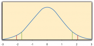
The reason the t statistic (or any test statistic) is useful is that we know how it is distributed when the null hypothesis is true. As shown in Figure 13.1, this distribution is unimodal and symmetrical, and it has a mean of 0. Its precise shape depends on a statistical concept called the degrees of freedom, which for a one-sample t -test is N − 1. (There are 24 degrees of freedom for the distribution shown in Figure 13.1.) The important point is that knowing this distribution makes it possible to find the p value for any t score. Consider, for example, a t score of 1.50 based on a sample of 25. The probability of a t score at least this extreme is given by the proportion of t scores in the distribution that are at least this extreme. For now, let us define extreme as being far from zero in either direction. Thus the p value is the proportion of t scores that are 1.50 or above or that are −1.50 or below—a value that turns out to be .14.
Fortunately, we do not have to deal directly with the distribution of t scores. If we were to enter our sample data and hypothetical mean of interest into one of the online statistical tools in Chapter 12 or into a program like SPSS (Excel does not have a one-sample t- test function), the output would include both the t score and the p value. At this point, the rest of the procedure is simple. If p is equal to or less than .05, we reject the null hypothesis and conclude that the population mean differs from the hypothetical mean of interest. If p is greater than .05, we retain the null hypothesis and conclude that there is not enough evidence to say that the population mean differs from the hypothetical mean of interest. (Again, technically, we conclude only that we do not have enough evidence to conclude that it does differ.)
If we were to compute the t score by hand, we could use a table like Table 13.2 to make the decision. This table does not provide actual p values. Instead, it provides the critical values of t for different degrees of freedom ( df) when α is .05. For now, let us focus on the two-tailed critical values in the last column of the table. Each of these values should be interpreted as a pair of values: one positive and one negative. For example, the two-tailed critical values when there are 24 degrees of freedom are 2.064 and −2.064. These are represented by the red vertical lines in Figure 13.1. The idea is that any t score below the lower critical value (the left-hand red line in Figure 13.1) is in the lowest 2.5% of the distribution, while any t score above the upper critical value (the right-hand red line) is in the highest 2.5% of the distribution. Therefore any t score beyond the critical value in either direction is in the most extreme 5% of t scores when the null hypothesis is true and has a p value less than .05. Thus if the t score we compute is beyond the critical value in either direction, then we reject the null hypothesis. If the t score we compute is between the upper and lower critical values, then we retain the null hypothesis.
| One-tailed | Two-tailed | |
| 3 | 2.353 | 3.182 |
| 4 | 2.132 | 2.776 |
| 5 | 2.015 | 2.571 |
| 6 | 1.943 | 2.447 |
| 7 | 1.895 | 2.365 |
| 8 | 1.860 | 2.306 |
| 9 | 1.833 | 2.262 |
| 10 | 1.812 | 2.228 |
| 11 | 1.796 | 2.201 |
| 12 | 1.782 | 2.179 |
| 13 | 1.771 | 2.160 |
| 14 | 1.761 | 2.145 |
| 15 | 1.753 | 2.131 |
| 16 | 1.746 | 2.120 |
| 17 | 1.740 | 2.110 |
| 18 | 1.734 | 2.101 |
| 19 | 1.729 | 2.093 |
| 20 | 1.725 | 2.086 |
| 21 | 1.721 | 2.080 |
| 22 | 1.717 | 2.074 |
| 23 | 1.714 | 2.069 |
| 24 | 1.711 | 2.064 |
| 25 | 1.708 | 2.060 |
| 30 | 1.697 | 2.042 |
| 35 | 1.690 | 2.030 |
| 40 | 1.684 | 2.021 |
| 45 | 1.679 | 2.014 |
| 50 | 1.676 | 2.009 |
| 60 | 1.671 | 2.000 |
| 70 | 1.667 | 1.994 |
| 80 | 1.664 | 1.990 |
| 90 | 1.662 | 1.987 |
| 100 | 1.660 | 1.984 |
Thus far, we have considered what is called a two-tailed test , where we reject the null hypothesis if the t score for the sample is extreme in either direction. This test makes sense when we believe that the sample mean might differ from the hypothetical population mean but we do not have good reason to expect the difference to go in a particular direction. But it is also possible to do a one-tailed test , where we reject the null hypothesis only if the t score for the sample is extreme in one direction that we specify before collecting the data. This test makes sense when we have good reason to expect the sample mean will differ from the hypothetical population mean in a particular direction.
Here is how it works. Each one-tailed critical value in Table 13.2 can again be interpreted as a pair of values: one positive and one negative. A t score below the lower critical value is in the lowest 5% of the distribution, and a t score above the upper critical value is in the highest 5% of the distribution. For 24 degrees of freedom, these values are −1.711 and 1.711. (These are represented by the green vertical lines in Figure 13.1.) However, for a one-tailed test, we must decide before collecting data whether we expect the sample mean to be lower than the hypothetical population mean, in which case we would use only the lower critical value, or we expect the sample mean to be greater than the hypothetical population mean, in which case we would use only the upper critical value. Notice that we still reject the null hypothesis when the t score for our sample is in the most extreme 5% of the t scores we would expect if the null hypothesis were true—so α remains at .05. We have simply redefined extreme to refer only to one tail of the distribution. The advantage of the one-tailed test is that critical values are less extreme. If the sample mean differs from the hypothetical population mean in the expected direction, then we have a better chance of rejecting the null hypothesis. The disadvantage is that if the sample mean differs from the hypothetical population mean in the unexpected direction, then there is no chance at all of rejecting the null hypothesis.
Example One-Sample t – Test
Imagine that a health psychologist is interested in the accuracy of university students’ estimates of the number of calories in a chocolate chip cookie. He shows the cookie to a sample of 10 students and asks each one to estimate the number of calories in it. Because the actual number of calories in the cookie is 250, this is the hypothetical population mean of interest (µ 0 ). The null hypothesis is that the mean estimate for the population (μ) is 250. Because he has no real sense of whether the students will underestimate or overestimate the number of calories, he decides to do a two-tailed test. Now imagine further that the participants’ actual estimates are as follows:
250, 280, 200, 150, 175, 200, 200, 220, 180, 250.
The mean estimate for the sample ( M ) is 212.00 calories and the standard deviation ( SD ) is 39.17. The health psychologist can now compute the t score for his sample:
[latex]t=\dfrac{{212-250}}{\left(\dfrac{39.17}{\sqrt10}\right)}=-3.07[/latex]
If he enters the data into one of the online analysis tools or uses SPSS, it would also tell him that the two-tailed p value for this t score (with 10 − 1 = 9 degrees of freedom) is .013. Because this is less than .05, the health psychologist would reject the null hypothesis and conclude that university students tend to underestimate the number of calories in a chocolate chip cookie. If he computes the t score by hand, he could look at Table 13.2 and see that the critical value of t for a two-tailed test with 9 degrees of freedom is ±2.262. The fact that his t score was more extreme than this critical value would tell him that his p value is less than .05 and that he should reject the null hypothesis. Using APA style, these results would be reported as follows: t (9) = -3.07, p = .01. Note that the t and p are italicized, the degrees of freedom appear in brackets with no decimal remainder, and the values of t and p are rounded to two decimal places.
Finally, if this researcher had gone into this study with good reason to expect that university students underestimate the number of calories, then he could have done a one-tailed test instead of a two-tailed test. The only thing this decision would change is the critical value, which would be −1.833. This slightly less extreme value would make it a bit easier to reject the null hypothesis. However, if it turned out that university students overestimate the number of calories—no matter how much they overestimate it—the researcher would not have been able to reject the null hypothesis.
The Dependent-Samples t – Test
The dependent-samples t -test (sometimes called the paired-samples t- test) is used to compare two means for the same sample tested at two different times or under two different conditions. This comparison is appropriate for pretest-posttest designs or within-subjects experiments. The null hypothesis is that the means at the two times or under the two conditions are the same in the population. The alternative hypothesis is that they are not the same. This test can also be one-tailed if the researcher has good reason to expect the difference goes in a particular direction.
It helps to think of the dependent-samples t- test as a special case of the one-sample t- test. However, the first step in the dependent-samples t- test is to reduce the two scores for each participant to a single difference score by taking the difference between them. At this point, the dependent-samples t- test becomes a one-sample t- test on the difference scores. The hypothetical population mean (µ 0 ) of interest is 0 because this is what the mean difference score would be if there were no difference on average between the two times or two conditions. We can now think of the null hypothesis as being that the mean difference score in the population is 0 (µ 0 = 0) and the alternative hypothesis as being that the mean difference score in the population is not 0 (µ 0 ≠ 0).
Example Dependent-Samples t – Test
Imagine that the health psychologist now knows that people tend to underestimate the number of calories in junk food and has developed a short training program to improve their estimates. To test the effectiveness of this program, he conducts a pretest-posttest study in which 10 participants estimate the number of calories in a chocolate chip cookie before the training program and then again afterward. Because he expects the program to increase the participants’ estimates, he decides to do a one-tailed test. Now imagine further that the pretest estimates are
230, 250, 280, 175, 150, 200, 180, 210, 220, 190
and that the posttest estimates (for the same participants in the same order) are
250, 260, 250, 200, 160, 200, 200, 180, 230, 240.
The difference scores, then, are as follows:
20, 10, −30, 25, 10, 0, 20, −30, 10, 50.
Note that it does not matter whether the first set of scores is subtracted from the second or the second from the first as long as it is done the same way for all participants. In this example, it makes sense to subtract the pretest estimates from the posttest estimates so that positive difference scores mean that the estimates went up after the training and negative difference scores mean the estimates went down.
The mean of the difference scores is 8.50 with a standard deviation of 27.27. The health psychologist can now compute the t score for his sample as follows:
[latex]t=\dfrac{{8.5-0}}{\left(\dfrac{27.27}{\sqrt10}\right)}=1.11[/latex]
If he enters the data into one of the online analysis tools or uses Excel or SPSS, it would tell him that the one-tailed p value for this t score (again with 10 − 1 = 9 degrees of freedom) is .148. Because this is greater than .05, he would retain the null hypothesis and conclude that the training program does not significantly increase people’s calorie estimates. If he were to compute the t score by hand, he could look at Table 13.2 and see that the critical value of t for a one-tailed test with 9 degrees of freedom is 1.833. (It is positive this time because he was expecting a positive mean difference score.) The fact that his t score was less extreme than this critical value would tell him that his p value is greater than .05 and that he should fail to reject the null hypothesis.
The Independent-Samples t- Test
The independent-samples t- test is used to compare the means of two separate samples ( M 1 and M 2 ). The two samples might have been tested under different conditions in a between-subjects experiment, or they could be pre-existing groups in a cross-sectional design (e.g., women and men, extraverts and introverts). The null hypothesis is that the means of the two populations are the same: µ 1 = µ 2 . The alternative hypothesis is that they are not the same: µ 1 ≠ µ 2 . Again, the test can be one-tailed if the researcher has good reason to expect the difference goes in a particular direction.
The t statistic here is a bit more complicated because it must take into account two sample means, two standard deviations, and two sample sizes. The formula is as follows:
[latex]t=\dfrac{{M{_1}-M{_2}}}{\sqrt{\dfrac{SD{^2}{_1}}{n{_1}}+\dfrac{SD{^2}{_2}}{n{_2}}}}[/latex]
Notice that this formula includes squared standard deviations (the variances) that appear inside the square root symbol. Also, lowercase n 1 and n 2 refer to the sample sizes in the two groups or condition (as opposed to capital N , which generally refers to the total sample size). The only additional thing to know here is that there are N − 2 degrees of freedom for the independent-samples t- test.
Example Independent-Samples t – Test
Now the health psychologist wants to compare the calorie estimates of people who regularly eat junk food with the estimates of people who rarely eat junk food. He believes the difference could come out in either direction so he decides to conduct a two-tailed test. He collects data from a sample of eight participants who eat junk food regularly and seven participants who rarely eat junk food. The data are as follows:
Junk food eaters: 180, 220, 150, 85, 200, 170, 150, 190
Non–junk food eaters: 200, 240, 190, 175, 200, 300, 240
The mean for the non-junk food eaters is 220.71 with a standard deviation of 41.23. The mean for the junk food eaters is 168.12 with a standard deviation of 42.66. He can now compute his t score as follows:
[latex]t=\dfrac{{220.71-168.12}}{\sqrt{\dfrac{41.23{^2}}{8}+\dfrac{42.66{^2}}{7}}}= 2.42[/latex]
If he enters the data into one of the online analysis tools or uses Excel or SPSS, it would tell him that the two-tailed p value for this t score (with 15 − 2 = 13 degrees of freedom) is .015. Because this p value is less than .05, the health psychologist would reject the null hypothesis and conclude that people who eat junk food regularly make lower calorie estimates than people who eat it rarely. If he were to compute the t score by hand, he could look at Table 13.2 and see that the critical value of t for a two-tailed test with 13 degrees of freedom is ±2.160. The fact that his t score was more extreme than this critical value would tell him that his p value is less than .05 and that he should reject the null hypothesis.
The Analysis of Variance
T -tests are used to compare two means (a sample mean with a population mean, the means of two conditions or two groups). When there are more than two groups or condition means to be compared, the most common null hypothesis test is the analysis of variance (ANOVA) . In this section, we look primarily at the one-way ANOVA , which is used for between-subjects designs with a single independent variable. We then briefly consider some other versions of the ANOVA that are used for within-subjects and factorial research designs.
One-Way ANOVA
The one-way ANOVA is used to compare the means of more than two samples ( M 1 , M 2 … M G ) in a between-subjects design. The null hypothesis is that all the means are equal in the population: µ 1 = µ 2 =…= µ G . The alternative hypothesis is that not all the means in the population are equal.
The test statistic for the ANOVA is called F . It is a ratio of two estimates of the population variance based on the sample data. One estimate of the population variance is called the mean squares between groups (MS B ) and is based on the differences among the sample means. The other is called the mean squares within groups (MS W ) and is based on the differences among the scores within each group. The F statistic is the ratio of the MS B to the MS W and can, therefore, be expressed as follows:
F = MS B / MS W
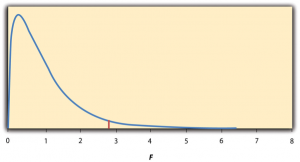
Again, the reason that F is useful is that we know how it is distributed when the null hypothesis is true. As shown in Figure 13.2, this distribution is unimodal and positively skewed with values that cluster around 1. The precise shape of the distribution depends on both the number of groups and the sample size, and there are degrees of freedom values associated with each of these. The between-groups degrees of freedom is the number of groups minus one: df B = ( G − 1). The within-groups degrees of freedom is the total sample size minus the number of groups: df W = N − G . Again, knowing the distribution of F when the null hypothesis is true allows us to find the p value.
The online tools in Chapter 12 and statistical software such as Excel and SPSS will compute F and find the p value. If p is equal to or less than .05, then we reject the null hypothesis and conclude that there are differences among the group means in the population. If p is greater than .05, then we retain the null hypothesis and conclude that there is not enough evidence to say that there are differences. In the unlikely event that we would compute F by hand, we can use a table of critical values like Table 13.3 “Table of Critical Values of ” to make the decision. The idea is that any F ratio greater than the critical value has a p value of less than .05. Thus if the F ratio we compute is beyond the critical value, then we reject the null hypothesis. If the F ratio we compute is less than the critical value, then we retain the null hypothesis.
| 2 | 3 | 4 | |
| 8 | 4.459 | 4.066 | 3.838 |
| 9 | 4.256 | 3.863 | 3.633 |
| 10 | 4.103 | 3.708 | 3.478 |
| 11 | 3.982 | 3.587 | 3.357 |
| 12 | 3.885 | 3.490 | 3.259 |
| 13 | 3.806 | 3.411 | 3.179 |
| 14 | 3.739 | 3.344 | 3.112 |
| 15 | 3.682 | 3.287 | 3.056 |
| 16 | 3.634 | 3.239 | 3.007 |
| 17 | 3.592 | 3.197 | 2.965 |
| 18 | 3.555 | 3.160 | 2.928 |
| 19 | 3.522 | 3.127 | 2.895 |
| 20 | 3.493 | 3.098 | 2.866 |
| 21 | 3.467 | 3.072 | 2.840 |
| 22 | 3.443 | 3.049 | 2.817 |
| 23 | 3.422 | 3.028 | 2.796 |
| 24 | 3.403 | 3.009 | 2.776 |
| 25 | 3.385 | 2.991 | 2.759 |
| 30 | 3.316 | 2.922 | 2.690 |
| 35 | 3.267 | 2.874 | 2.641 |
| 40 | 3.232 | 2.839 | 2.606 |
| 45 | 3.204 | 2.812 | 2.579 |
| 50 | 3.183 | 2.790 | 2.557 |
| 55 | 3.165 | 2.773 | 2.540 |
| 60 | 3.150 | 2.758 | 2.525 |
| 65 | 3.138 | 2.746 | 2.513 |
| 70 | 3.128 | 2.736 | 2.503 |
| 75 | 3.119 | 2.727 | 2.494 |
| 80 | 3.111 | 2.719 | 2.486 |
| 85 | 3.104 | 2.712 | 2.479 |
| 90 | 3.098 | 2.706 | 2.473 |
| 95 | 3.092 | 2.700 | 2.467 |
| 100 | 3.087 | 2.696 | 2.463 |
Example One-Way ANOVA
Imagine that the health psychologist wants to compare the calorie estimates of psychology majors, nutrition majors, and professional dieticians. He collects the following data:
Psych majors: 200, 180, 220, 160, 150, 200, 190, 200
Nutrition majors: 190, 220, 200, 230, 160, 150, 200, 210, 195
Dieticians: 220, 250, 240, 275, 250, 230, 200, 240
The means are 187.50 ( SD = 23.14), 195.00 ( SD = 27.77), and 238.13 ( SD = 22.35), respectively. So it appears that dieticians made substantially more accurate estimates on average. The researcher would almost certainly enter these data into a program such as Excel or SPSS, which would compute F for him or her and find the p value. Table 13.4 shows the output of the one-way ANOVA function in Excel for these data. This table is referred to as an ANOVA table. It shows that MS B is 5,971.88, MS W is 602.23, and their ratio, F , is 9.92. The p value is .0009. Because this value is below .05, the researcher would reject the null hypothesis and conclude that the mean calorie estimates for the three groups are not the same in the population. Notice that the ANOVA table also includes the “sum of squares” ( SS ) for between groups and for within groups. These values are computed on the way to finding MS B and MS W but are not typically reported by the researcher. Finally, if the researcher were to compute the F ratio by hand, he could look at Table 13.3 and see that the critical value of F with 2 and 21 degrees of freedom is 3.467 (the same value in Table 13.4 under F crit ). The fact that his F score was more extreme than this critical value would tell him that his p value is less than .05 and that he should reject the null hypothesis.
| Between groups | 11,943.75 | 2 | 5,971.875 | 9.916234 | 0.000928 | 3.4668 |
| Within groups | 12,646.88 | 21 | 602.2321 | |||
| Total | 24,590.63 | 23 | ||||
ANOVA Elaborations
Post hoc comparisons.
When we reject the null hypothesis in a one-way ANOVA, we conclude that the group means are not all the same in the population. But this can indicate different things. With three groups, it can indicate that all three means are significantly different from each other. Or it can indicate that one of the means is significantly different from the other two, but the other two are not significantly different from each other. It could be, for example, that the mean calorie estimates of psychology majors, nutrition majors, and dieticians are all significantly different from each other. Or it could be that the mean for dieticians is significantly different from the means for psychology and nutrition majors, but the means for psychology and nutrition majors are not significantly different from each other. For this reason, statistically significant one-way ANOVA results are typically followed up with a series of post hoc comparisons of selected pairs of group means to determine which are different from which others.
One approach to post hoc comparisons would be to conduct a series of independent-samples t- tests comparing each group mean to each of the other group means. But there is a problem with this approach. In general, if we conduct a t -test when the null hypothesis is true, we have a 5% chance of mistakenly rejecting the null hypothesis (see Section 13.3 “Additional Considerations” for more on such Type I errors). If we conduct several t- tests when the null hypothesis is true, the chance of mistakenly rejecting at least one null hypothesis increases with each test we conduct. Thus researchers do not usually make post hoc comparisons using standard t- tests because there is too great a chance that they will mistakenly reject at least one null hypothesis. Instead, they use one of several modified t -test procedures—among them the Bonferonni procedure, Fisher’s least significant difference (LSD) test, and Tukey’s honestly significant difference (HSD) test. The details of these approaches are beyond the scope of this book, but it is important to understand their purpose. It is to keep the risk of mistakenly rejecting a true null hypothesis to an acceptable level (close to 5%).
Repeated-Measures ANOVA
Recall that the one-way ANOVA is appropriate for between-subjects designs in which the means being compared come from separate groups of participants. It is not appropriate for within-subjects designs in which the means being compared come from the same participants tested under different conditions or at different times. This requires a slightly different approach, called the repeated-measures ANOVA . The basics of the repeated-measures ANOVA are the same as for the one-way ANOVA. The main difference is that measuring the dependent variable multiple times for each participant allows for a more refined measure of MS W . Imagine, for example, that the dependent variable in a study is a measure of reaction time. Some participants will be faster or slower than others because of stable individual differences in their nervous systems, muscles, and other factors. In a between-subjects design, these stable individual differences would simply add to the variability within the groups and increase the value of MS W (which would, in turn, decrease the value of F). In a within-subjects design, however, these stable individual differences can be measured and subtracted from the value of MS W . This lower value of MS W means a higher value of F and a more sensitive test.
Factorial ANOVA
When more than one independent variable is included in a factorial design, the appropriate approach is the factorial ANOVA . Again, the basics of the factorial ANOVA are the same as for the one-way and repeated-measures ANOVAs. The main difference is that it produces an F ratio and p value for each main effect and for each interaction. Returning to our calorie estimation example, imagine that the health psychologist tests the effect of participant major (psychology vs. nutrition) and food type (cookie vs. hamburger) in a factorial design. A factorial ANOVA would produce separate F ratios and p values for the main effect of major, the main effect of food type, and the interaction between major and food. Appropriate modifications must be made depending on whether the design is between-subjects, within-subjects, or mixed.
Testing Correlation Coefficients
For relationships between quantitative variables, where Pearson’s r (the correlation coefficient) is used to describe the strength of those relationships, the appropriate null hypothesis test is a test of the correlation coefficient. The basic logic is exactly the same as for other null hypothesis tests. In this case, the null hypothesis is that there is no relationship in the population. We can use the Greek lowercase rho (ρ) to represent the relevant parameter: ρ = 0. The alternative hypothesis is that there is a relationship in the population: ρ ≠ 0. As with the t- test, this test can be two-tailed if the researcher has no expectation about the direction of the relationship or one-tailed if the researcher expects the relationship to go in a particular direction.
It is possible to use the correlation coefficient for the sample to compute a t score with N − 2 degrees of freedom and then to proceed as for a t- test. However, because of the way it is computed, the correlation coefficient can also be treated as its own test statistic. The online statistical tools and statistical software such as Excel and SPSS generally compute the correlation coefficient and provide the p value associated with that value. As always, if the p value is equal to or less than .05, we reject the null hypothesis and conclude that there is a relationship between the variables in the population. If the p value is greater than .05, we retain the null hypothesis and conclude that there is not enough evidence to say there is a relationship in the population. If we compute the correlation coefficient by hand, we can use a table like Table 13.5, which shows the critical values of r for various samples sizes when α is .05. A sample value of the correlation coefficient that is more extreme than the critical value is statistically significant.
| One-tailed | Two-tailed | |
| 5 | .805 | .878 |
| 10 | .549 | .632 |
| 15 | .441 | .514 |
| 20 | .378 | .444 |
| 25 | .337 | .396 |
| 30 | .306 | .361 |
| 35 | .283 | .334 |
| 40 | .264 | .312 |
| 45 | .248 | .294 |
| 50 | .235 | .279 |
| 55 | .224 | .266 |
| 60 | .214 | .254 |
| 65 | .206 | .244 |
| 70 | .198 | .235 |
| 75 | .191 | .227 |
| 80 | .185 | .220 |
| 85 | .180 | .213 |
| 90 | .174 | .207 |
| 95 | .170 | .202 |
| 100 | .165 | .197 |
Example Test of a Correlation Coefficient
Imagine that the health psychologist is interested in the correlation between people’s calorie estimates and their weight. She has no expectation about the direction of the relationship, so she decides to conduct a two-tailed test. She computes the correlation coefficient for a sample of 22 university students and finds that Pearson’s r is −.21. The statistical software she uses tells her that the p value is .348. It is greater than .05, so she retains the null hypothesis and concludes that there is no relationship between people’s calorie estimates and their weight. If she were to compute the correlation coefficient by hand, she could look at Table 13.5 and see that the critical value for 22 − 2 = 20 degrees of freedom is .444. The fact that the correlation coefficient for her sample is less extreme than this critical value tells her that the p value is greater than .05 and that she should retain the null hypothesis.
A test that involves looking at the difference between two means.
Used to compare a sample mean (M) with a hypothetical population mean (μ0) that provides some interesting standard of comparison.
A statistic (e.g., F , t , etc.) that is computed to compare against what is expected in the null hypothesis, and thus helps find the p value.
The absolute value that a test statistic (e.g., F , t , etc.) must exceed to be considered statistically significant.
Where we reject the null hypothesis if the test statistic for the sample is extreme in either direction (+/-).
Where we reject the null hypothesis only if the t score for the sample is extreme in one direction that we specify before collecting the data.
Used to compare two means for the same sample tested at two different times or under two different conditions (sometimes called the paired-samples t -test).
A method to reduce pairs of scores (e.g., pre- and post-test) to a single score by calculating the difference between them.
Used to compare the means of two separate samples (M1 and M2).
A statistical test used when there are more than two groups or condition means to be compared.
Used for between-subjects designs with a single independent variable.
An estimate of the population variance and is based on the differences among the sample means.
An estimate of the population variance and is based on the differences among the scores within each group.
An unplanned (not hypothesized) test of which pairs of group mean scores are different from which others.
Compares the means from the same participants tested under different conditions or at different times in which the dependent variable is measured multiple times for each participant.
A statistical method to detect differences in the means between conditions when there are two or more independent variables in a factorial design. It allows the detection of main effects and interaction effects.
Research Methods in Psychology Copyright © 2019 by Rajiv S. Jhangiani, I-Chant A. Chiang, Carrie Cuttler, & Dana C. Leighton is licensed under a Creative Commons Attribution-NonCommercial-ShareAlike 4.0 International License , except where otherwise noted.
Share This Book
Have a language expert improve your writing
Run a free plagiarism check in 10 minutes, generate accurate citations for free.
- Knowledge Base
- Null and Alternative Hypotheses | Definitions & Examples
Null & Alternative Hypotheses | Definitions, Templates & Examples
Published on May 6, 2022 by Shaun Turney . Revised on June 22, 2023.
The null and alternative hypotheses are two competing claims that researchers weigh evidence for and against using a statistical test :
- Null hypothesis ( H 0 ): There’s no effect in the population .
- Alternative hypothesis ( H a or H 1 ) : There’s an effect in the population.
Table of contents
Answering your research question with hypotheses, what is a null hypothesis, what is an alternative hypothesis, similarities and differences between null and alternative hypotheses, how to write null and alternative hypotheses, other interesting articles, frequently asked questions.
The null and alternative hypotheses offer competing answers to your research question . When the research question asks “Does the independent variable affect the dependent variable?”:
- The null hypothesis ( H 0 ) answers “No, there’s no effect in the population.”
- The alternative hypothesis ( H a ) answers “Yes, there is an effect in the population.”
The null and alternative are always claims about the population. That’s because the goal of hypothesis testing is to make inferences about a population based on a sample . Often, we infer whether there’s an effect in the population by looking at differences between groups or relationships between variables in the sample. It’s critical for your research to write strong hypotheses .
You can use a statistical test to decide whether the evidence favors the null or alternative hypothesis. Each type of statistical test comes with a specific way of phrasing the null and alternative hypothesis. However, the hypotheses can also be phrased in a general way that applies to any test.
Receive feedback on language, structure, and formatting
Professional editors proofread and edit your paper by focusing on:
- Academic style
- Vague sentences
- Style consistency
See an example

The null hypothesis is the claim that there’s no effect in the population.
If the sample provides enough evidence against the claim that there’s no effect in the population ( p ≤ α), then we can reject the null hypothesis . Otherwise, we fail to reject the null hypothesis.
Although “fail to reject” may sound awkward, it’s the only wording that statisticians accept . Be careful not to say you “prove” or “accept” the null hypothesis.
Null hypotheses often include phrases such as “no effect,” “no difference,” or “no relationship.” When written in mathematical terms, they always include an equality (usually =, but sometimes ≥ or ≤).
You can never know with complete certainty whether there is an effect in the population. Some percentage of the time, your inference about the population will be incorrect. When you incorrectly reject the null hypothesis, it’s called a type I error . When you incorrectly fail to reject it, it’s a type II error.
Examples of null hypotheses
The table below gives examples of research questions and null hypotheses. There’s always more than one way to answer a research question, but these null hypotheses can help you get started.
| ( ) | ||
| Does tooth flossing affect the number of cavities? | Tooth flossing has on the number of cavities. | test: The mean number of cavities per person does not differ between the flossing group (µ ) and the non-flossing group (µ ) in the population; µ = µ . |
| Does the amount of text highlighted in the textbook affect exam scores? | The amount of text highlighted in the textbook has on exam scores. | : There is no relationship between the amount of text highlighted and exam scores in the population; β = 0. |
| Does daily meditation decrease the incidence of depression? | Daily meditation the incidence of depression.* | test: The proportion of people with depression in the daily-meditation group ( ) is greater than or equal to the no-meditation group ( ) in the population; ≥ . |
*Note that some researchers prefer to always write the null hypothesis in terms of “no effect” and “=”. It would be fine to say that daily meditation has no effect on the incidence of depression and p 1 = p 2 .
The alternative hypothesis ( H a ) is the other answer to your research question . It claims that there’s an effect in the population.
Often, your alternative hypothesis is the same as your research hypothesis. In other words, it’s the claim that you expect or hope will be true.
The alternative hypothesis is the complement to the null hypothesis. Null and alternative hypotheses are exhaustive, meaning that together they cover every possible outcome. They are also mutually exclusive, meaning that only one can be true at a time.
Alternative hypotheses often include phrases such as “an effect,” “a difference,” or “a relationship.” When alternative hypotheses are written in mathematical terms, they always include an inequality (usually ≠, but sometimes < or >). As with null hypotheses, there are many acceptable ways to phrase an alternative hypothesis.
Examples of alternative hypotheses
The table below gives examples of research questions and alternative hypotheses to help you get started with formulating your own.
| Does tooth flossing affect the number of cavities? | Tooth flossing has an on the number of cavities. | test: The mean number of cavities per person differs between the flossing group (µ ) and the non-flossing group (µ ) in the population; µ ≠ µ . |
| Does the amount of text highlighted in a textbook affect exam scores? | The amount of text highlighted in the textbook has an on exam scores. | : There is a relationship between the amount of text highlighted and exam scores in the population; β ≠ 0. |
| Does daily meditation decrease the incidence of depression? | Daily meditation the incidence of depression. | test: The proportion of people with depression in the daily-meditation group ( ) is less than the no-meditation group ( ) in the population; < . |
Null and alternative hypotheses are similar in some ways:
- They’re both answers to the research question.
- They both make claims about the population.
- They’re both evaluated by statistical tests.
However, there are important differences between the two types of hypotheses, summarized in the following table.
| A claim that there is in the population. | A claim that there is in the population. | |
|
| ||
| Equality symbol (=, ≥, or ≤) | Inequality symbol (≠, <, or >) | |
| Rejected | Supported | |
| Failed to reject | Not supported |
Prevent plagiarism. Run a free check.
To help you write your hypotheses, you can use the template sentences below. If you know which statistical test you’re going to use, you can use the test-specific template sentences. Otherwise, you can use the general template sentences.
General template sentences
The only thing you need to know to use these general template sentences are your dependent and independent variables. To write your research question, null hypothesis, and alternative hypothesis, fill in the following sentences with your variables:
Does independent variable affect dependent variable ?
- Null hypothesis ( H 0 ): Independent variable does not affect dependent variable.
- Alternative hypothesis ( H a ): Independent variable affects dependent variable.
Test-specific template sentences
Once you know the statistical test you’ll be using, you can write your hypotheses in a more precise and mathematical way specific to the test you chose. The table below provides template sentences for common statistical tests.
| ( ) | ||
| test
with two groups | The mean dependent variable does not differ between group 1 (µ ) and group 2 (µ ) in the population; µ = µ . | The mean dependent variable differs between group 1 (µ ) and group 2 (µ ) in the population; µ ≠ µ . |
| with three groups | The mean dependent variable does not differ between group 1 (µ ), group 2 (µ ), and group 3 (µ ) in the population; µ = µ = µ . | The mean dependent variable of group 1 (µ ), group 2 (µ ), and group 3 (µ ) are not all equal in the population. |
| There is no correlation between independent variable and dependent variable in the population; ρ = 0. | There is a correlation between independent variable and dependent variable in the population; ρ ≠ 0. | |
| There is no relationship between independent variable and dependent variable in the population; β = 0. | There is a relationship between independent variable and dependent variable in the population; β ≠ 0. | |
| Two-proportions test | The dependent variable expressed as a proportion does not differ between group 1 ( ) and group 2 ( ) in the population; = . | The dependent variable expressed as a proportion differs between group 1 ( ) and group 2 ( ) in the population; ≠ . |
Note: The template sentences above assume that you’re performing one-tailed tests . One-tailed tests are appropriate for most studies.
If you want to know more about statistics , methodology , or research bias , make sure to check out some of our other articles with explanations and examples.
- Normal distribution
- Descriptive statistics
- Measures of central tendency
- Correlation coefficient
Methodology
- Cluster sampling
- Stratified sampling
- Types of interviews
- Cohort study
- Thematic analysis
Research bias
- Implicit bias
- Cognitive bias
- Survivorship bias
- Availability heuristic
- Nonresponse bias
- Regression to the mean
Hypothesis testing is a formal procedure for investigating our ideas about the world using statistics. It is used by scientists to test specific predictions, called hypotheses , by calculating how likely it is that a pattern or relationship between variables could have arisen by chance.
Null and alternative hypotheses are used in statistical hypothesis testing . The null hypothesis of a test always predicts no effect or no relationship between variables, while the alternative hypothesis states your research prediction of an effect or relationship.
The null hypothesis is often abbreviated as H 0 . When the null hypothesis is written using mathematical symbols, it always includes an equality symbol (usually =, but sometimes ≥ or ≤).
The alternative hypothesis is often abbreviated as H a or H 1 . When the alternative hypothesis is written using mathematical symbols, it always includes an inequality symbol (usually ≠, but sometimes < or >).
A research hypothesis is your proposed answer to your research question. The research hypothesis usually includes an explanation (“ x affects y because …”).
A statistical hypothesis, on the other hand, is a mathematical statement about a population parameter. Statistical hypotheses always come in pairs: the null and alternative hypotheses . In a well-designed study , the statistical hypotheses correspond logically to the research hypothesis.
Cite this Scribbr article
If you want to cite this source, you can copy and paste the citation or click the “Cite this Scribbr article” button to automatically add the citation to our free Citation Generator.
Turney, S. (2023, June 22). Null & Alternative Hypotheses | Definitions, Templates & Examples. Scribbr. Retrieved July 10, 2024, from https://www.scribbr.com/statistics/null-and-alternative-hypotheses/
Is this article helpful?

Shaun Turney
Other students also liked, inferential statistics | an easy introduction & examples, hypothesis testing | a step-by-step guide with easy examples, type i & type ii errors | differences, examples, visualizations, what is your plagiarism score.
Introduction to Hypothesis Testing (Psychology)
Contents Toggle Main Menu 1 What is a Hypothesis test? 2 The Null and Alternative Hypotheses 3 The Structure of a Hypothesis Test 3.1 Summary of Steps for a Hypothesis Test 4 P -Values 5 Parametric and Non-Parametric Hypothesis Tests 6 One and two tailed tests 7 Type I and Type II Errors 8 See Also 9 Worksheets
What is a Hypothesis test?
A statistical hypothesis is an unproven statement which can be tested. A hypothesis test is used to test whether this statement is true.
The Null and Alternative Hypotheses
- The null hypothesis $H_0$, is where you assume that the observations are statistically independent i.e. no difference in the populations you are testing. If the null hypothesis is true, it suggests that any changes witnessed in an experiment are because of random chance and not because of changes made to variables in the experiment. For example, serotonin levels have no effect on ability to cope with stress. See also Null and alternative hypotheses .
- The alternative hypothesis $H_1$, is a theory that the observations are related (not independent) in some way. We only adopt the alternative hypothesis if we have rejected the null hypothesis. For example, serotonin levels affect a person's ability to cope with stress. You do not necessarily have to specify in what way they are related but can do (see one and two tailed tests for more information).
The Structure of a Hypothesis Test
- The first step of a hypothesis test is to state the null hypothesis $H_0$ and the alternative hypothesis $H_1$ . The null hypothesis is the statement or claim being made (which we are trying to disprove) and the alternative hypothesis is the hypothesis that we are trying to prove and which is accepted if we have sufficient evidence to reject the null hypothesis.
For example, consider a person in court who is charged with murder. The jury needs to decide whether the person in innocent (the null hypothesis) or guilty (the alternative hypothesis). As usual, we assume the person is innocent unless the jury can provide sufficient evidence that the person is guilty. Similarly, we assume that $H_0$ is true unless we can provide sufficient evidence that it is false and that $H_1$ is true, in which case we reject $H_0$ and accept $H_1$.
To decide if we have sufficient evidence against the null hypothesis to reject it (in favour of the alternative hypothesis), we must first decide upon a significance level . The significance level is the probability of rejecting the null hypothesis when it the null hypothesis is true and is denoted by $\alpha$. The $5\%$ significance level is a common choice for statistical test.
The next step is to collect data and calculate the test statistic and associated $p$-value using the data. Assuming that the null hypothesis is true, the $p$-value is the probability of obtaining a sample statistic equal to or more extreme than the observed test statistic.
Next we must compare the $p$-value with the chosen significance level. If $p \lt \alpha$ then we reject $H_0$ and accept $H_1$. The lower $p$, the more evidence we have against $H_0$ and so the more confidence we can have that $H_0$ is false. If $p \geq \alpha$ then we do not have sufficient evidence to reject the $H_0$ and so must accept it.
Alternatively, we can compare our test statistic with the appropriate critical value for the chosen significance level. We can look up critical values in distribution tables (see worked examples below). If our test statistic is:
- positive and greater than the critical value, then we have sufficient evidence to reject the null hypothesis and accept the alternative hypothesis.
- positive and lower than or equal to the critical value, we must accept the null hypothesis.
- negative and lower than the critical value, then we have sufficient evidence to reject the null hypothesis and accept the alternative hypothesis.
- negative and greater than or equal to the critical value, we must accept the null hypothesis.
For either method:
Significant difference found: Reject the null hypothesis No significant difference found: Accept the null hypothesis
Finally, we must interpret our results and come to a conclusion. Returning to the example of the person in court, if the result of our hypothesis test indicated that we should accept $H_1$ and reject $H_0$, our conclusion would be that the jury should declare the person guilty of murder.
Summary of Steps for a Hypothesis Test
- Specify the null and the alternative hypothesis
- Decide upon the significance level.
- Comparing the $p$-value to the significance level $\alpha$, or
- Comparing the test statistic to the critical value.
- Interpret your results and draw a conclusion
P -Values"> P -Values
The $p$ -value is the probability of the test statistic (e.g. t -value or Chi-Square value) occurring given the null hypothesis is true. Since it is a probability, the $p$-value is a number between $0$ and $1$.
- Typically $p \leq 0.05$ shows that there is strong evidence for $H_1$ so we can accept it and reject $H_0$. Any $p$-value less than $0.05$ is significant and $p$-values less than $0.01$ are very significant .
- Typically $ p > 0.05$ shows that there is poor evidence for $H_1$ so we reject it and accept $H_0$.
- The smaller the $p$-value the more evidence there is supporting the hypothesis.
- The rule for accepting and rejecting the hypothesis is:
\begin{align} \text {Significant difference found} &= \textbf{Reject}\text{ the null hypothesis}\\ \text {No Significant difference found} &= \textbf{Accept}\text{ the null hypothesis}\\ \end{align}
- Note : The significance level is not always $0.05$. It can differ depending on the application and is often subjective (different people will have different opinions on what values are appropriate). For example, if lives are at stake then the $p$-value must be very small for safety reasons.
- See $P$-values for further detail on this topic.
Parametric and Non-Parametric Hypothesis Tests
There are parametric and non-parametric hypothesis tests.
- A parametric hypothesis assumes that the data follows a Normal probability distribution (with equal variances if we are working with more than one set of data) . A parametric hypothesis test is a statement about the parameters of this distribution (typically the mean). This can be seen in more detail in the Parametric Hypotheses Tests section .
- A non-parametric test assumes that the data does not follow any distribution and usually bases its calculations on the median . Note that although we assume the data does not follow a particular distribution it may do anyway. This can be seen in more detail in the Non-Parametric Hypotheses Tests section .
One and two tailed tests
Whether a test is One-tailed or Two-tailed is appropriate depends upon the alternative hypothesis $H_1$.
- One-tailed tests are used when the alternative hypothesis states that the parameter of interest is either bigger or smaller than the value stated in the null hypothesis. For example, the null hypothesis might state that the average weight of chocolate bars produced by a chocolate factory in Slough is 35g (as is printed on the wrapper), while the alternative hypothesis might state that the average weight of the chocolate bars is in fact lower than 35g.
- Two-tailed tests are used when the hypothesis states that the parameter of interest differs from the null hypothesis but does not specify in which direction. In the above example, a Two-tailed alternative hypothesis would be that the average weight of the chocolate bars is not equal to 35g.
Type I and Type II Errors
- A Type I error is made if we reject the null hypothesis when it is true (so should have been accepted). Returning to the example of the person in court, a Type I error would be made if the jury declared the person guilty when they are in fact innocent. The probability of making a Type I error is equal to the significance level $\alpha$.
- A Type II error is made if we accept the null hypothesis when it is false i.e. we should have rejected the null hypothesis and accepted the alternative hypothesis. This would occur if the jury declared the person innocent when they are in fact guilty.
For more information about the topics covered here see hypothesis testing .
- Introduction to hypothesis testing
- Binomial tests
Want to create or adapt books like this? Learn more about how Pressbooks supports open publishing practices.
Chapter 13: Inferential Statistics
Understanding Null Hypothesis Testing
Learning Objectives
- Explain the purpose of null hypothesis testing, including the role of sampling error.
- Describe the basic logic of null hypothesis testing.
- Describe the role of relationship strength and sample size in determining statistical significance and make reasonable judgments about statistical significance based on these two factors.
The Purpose of Null Hypothesis Testing
As we have seen, psychological research typically involves measuring one or more variables for a sample and computing descriptive statistics for that sample. In general, however, the researcher’s goal is not to draw conclusions about that sample but to draw conclusions about the population that the sample was selected from. Thus researchers must use sample statistics to draw conclusions about the corresponding values in the population. These corresponding values in the population are called parameters . Imagine, for example, that a researcher measures the number of depressive symptoms exhibited by each of 50 clinically depressed adults and computes the mean number of symptoms. The researcher probably wants to use this sample statistic (the mean number of symptoms for the sample) to draw conclusions about the corresponding population parameter (the mean number of symptoms for clinically depressed adults).
Unfortunately, sample statistics are not perfect estimates of their corresponding population parameters. This is because there is a certain amount of random variability in any statistic from sample to sample. The mean number of depressive symptoms might be 8.73 in one sample of clinically depressed adults, 6.45 in a second sample, and 9.44 in a third—even though these samples are selected randomly from the same population. Similarly, the correlation (Pearson’s r ) between two variables might be +.24 in one sample, −.04 in a second sample, and +.15 in a third—again, even though these samples are selected randomly from the same population. This random variability in a statistic from sample to sample is called sampling error . (Note that the term error here refers to random variability and does not imply that anyone has made a mistake. No one “commits a sampling error.”)
One implication of this is that when there is a statistical relationship in a sample, it is not always clear that there is a statistical relationship in the population. A small difference between two group means in a sample might indicate that there is a small difference between the two group means in the population. But it could also be that there is no difference between the means in the population and that the difference in the sample is just a matter of sampling error. Similarly, a Pearson’s r value of −.29 in a sample might mean that there is a negative relationship in the population. But it could also be that there is no relationship in the population and that the relationship in the sample is just a matter of sampling error.
In fact, any statistical relationship in a sample can be interpreted in two ways:
- There is a relationship in the population, and the relationship in the sample reflects this.
- There is no relationship in the population, and the relationship in the sample reflects only sampling error.
The purpose of null hypothesis testing is simply to help researchers decide between these two interpretations.
The Logic of Null Hypothesis Testing
Null hypothesis testing is a formal approach to deciding between two interpretations of a statistical relationship in a sample. One interpretation is called the null hypothesis (often symbolized H 0 and read as “H-naught”). This is the idea that there is no relationship in the population and that the relationship in the sample reflects only sampling error. Informally, the null hypothesis is that the sample relationship “occurred by chance.” The other interpretation is called the alternative hypothesis (often symbolized as H 1 ). This is the idea that there is a relationship in the population and that the relationship in the sample reflects this relationship in the population.
Again, every statistical relationship in a sample can be interpreted in either of these two ways: It might have occurred by chance, or it might reflect a relationship in the population. So researchers need a way to decide between them. Although there are many specific null hypothesis testing techniques, they are all based on the same general logic. The steps are as follows:
- Assume for the moment that the null hypothesis is true. There is no relationship between the variables in the population.
- Determine how likely the sample relationship would be if the null hypothesis were true.
- If the sample relationship would be extremely unlikely, then reject the null hypothesis in favour of the alternative hypothesis. If it would not be extremely unlikely, then retain the null hypothesis .
Following this logic, we can begin to understand why Mehl and his colleagues concluded that there is no difference in talkativeness between women and men in the population. In essence, they asked the following question: “If there were no difference in the population, how likely is it that we would find a small difference of d = 0.06 in our sample?” Their answer to this question was that this sample relationship would be fairly likely if the null hypothesis were true. Therefore, they retained the null hypothesis—concluding that there is no evidence of a sex difference in the population. We can also see why Kanner and his colleagues concluded that there is a correlation between hassles and symptoms in the population. They asked, “If the null hypothesis were true, how likely is it that we would find a strong correlation of +.60 in our sample?” Their answer to this question was that this sample relationship would be fairly unlikely if the null hypothesis were true. Therefore, they rejected the null hypothesis in favour of the alternative hypothesis—concluding that there is a positive correlation between these variables in the population.
A crucial step in null hypothesis testing is finding the likelihood of the sample result if the null hypothesis were true. This probability is called the p value . A low p value means that the sample result would be unlikely if the null hypothesis were true and leads to the rejection of the null hypothesis. A high p value means that the sample result would be likely if the null hypothesis were true and leads to the retention of the null hypothesis. But how low must the p value be before the sample result is considered unlikely enough to reject the null hypothesis? In null hypothesis testing, this criterion is called α (alpha) and is almost always set to .05. If there is less than a 5% chance of a result as extreme as the sample result if the null hypothesis were true, then the null hypothesis is rejected. When this happens, the result is said to be statistically significant . If there is greater than a 5% chance of a result as extreme as the sample result when the null hypothesis is true, then the null hypothesis is retained. This does not necessarily mean that the researcher accepts the null hypothesis as true—only that there is not currently enough evidence to conclude that it is true. Researchers often use the expression “fail to reject the null hypothesis” rather than “retain the null hypothesis,” but they never use the expression “accept the null hypothesis.”
The Misunderstood p Value
The p value is one of the most misunderstood quantities in psychological research (Cohen, 1994) [1] . Even professional researchers misinterpret it, and it is not unusual for such misinterpretations to appear in statistics textbooks!
The most common misinterpretation is that the p value is the probability that the null hypothesis is true—that the sample result occurred by chance. For example, a misguided researcher might say that because the p value is .02, there is only a 2% chance that the result is due to chance and a 98% chance that it reflects a real relationship in the population. But this is incorrect . The p value is really the probability of a result at least as extreme as the sample result if the null hypothesis were true. So a p value of .02 means that if the null hypothesis were true, a sample result this extreme would occur only 2% of the time.
You can avoid this misunderstanding by remembering that the p value is not the probability that any particular hypothesis is true or false. Instead, it is the probability of obtaining the sample result if the null hypothesis were true.
Role of Sample Size and Relationship Strength
Recall that null hypothesis testing involves answering the question, “If the null hypothesis were true, what is the probability of a sample result as extreme as this one?” In other words, “What is the p value?” It can be helpful to see that the answer to this question depends on just two considerations: the strength of the relationship and the size of the sample. Specifically, the stronger the sample relationship and the larger the sample, the less likely the result would be if the null hypothesis were true. That is, the lower the p value. This should make sense. Imagine a study in which a sample of 500 women is compared with a sample of 500 men in terms of some psychological characteristic, and Cohen’s d is a strong 0.50. If there were really no sex difference in the population, then a result this strong based on such a large sample should seem highly unlikely. Now imagine a similar study in which a sample of three women is compared with a sample of three men, and Cohen’s d is a weak 0.10. If there were no sex difference in the population, then a relationship this weak based on such a small sample should seem likely. And this is precisely why the null hypothesis would be rejected in the first example and retained in the second.
Of course, sometimes the result can be weak and the sample large, or the result can be strong and the sample small. In these cases, the two considerations trade off against each other so that a weak result can be statistically significant if the sample is large enough and a strong relationship can be statistically significant even if the sample is small. Table 13.1 shows roughly how relationship strength and sample size combine to determine whether a sample result is statistically significant. The columns of the table represent the three levels of relationship strength: weak, medium, and strong. The rows represent four sample sizes that can be considered small, medium, large, and extra large in the context of psychological research. Thus each cell in the table represents a combination of relationship strength and sample size. If a cell contains the word Yes , then this combination would be statistically significant for both Cohen’s d and Pearson’s r . If it contains the word No , then it would not be statistically significant for either. There is one cell where the decision for d and r would be different and another where it might be different depending on some additional considerations, which are discussed in Section 13.2 “Some Basic Null Hypothesis Tests”
| Sample Size | Weak relationship | Medium-strength relationship | Strong relationship |
|---|---|---|---|
| Small ( = 20) | No | No | = Maybe = Yes |
| Medium ( = 50) | No | Yes | Yes |
| Large ( = 100) | = Yes = No | Yes | Yes |
| Extra large ( = 500) | Yes | Yes | Yes |
Although Table 13.1 provides only a rough guideline, it shows very clearly that weak relationships based on medium or small samples are never statistically significant and that strong relationships based on medium or larger samples are always statistically significant. If you keep this lesson in mind, you will often know whether a result is statistically significant based on the descriptive statistics alone. It is extremely useful to be able to develop this kind of intuitive judgment. One reason is that it allows you to develop expectations about how your formal null hypothesis tests are going to come out, which in turn allows you to detect problems in your analyses. For example, if your sample relationship is strong and your sample is medium, then you would expect to reject the null hypothesis. If for some reason your formal null hypothesis test indicates otherwise, then you need to double-check your computations and interpretations. A second reason is that the ability to make this kind of intuitive judgment is an indication that you understand the basic logic of this approach in addition to being able to do the computations.
Statistical Significance Versus Practical Significance
Table 13.1 illustrates another extremely important point. A statistically significant result is not necessarily a strong one. Even a very weak result can be statistically significant if it is based on a large enough sample. This is closely related to Janet Shibley Hyde’s argument about sex differences (Hyde, 2007) [2] . The differences between women and men in mathematical problem solving and leadership ability are statistically significant. But the word significant can cause people to interpret these differences as strong and important—perhaps even important enough to influence the college courses they take or even who they vote for. As we have seen, however, these statistically significant differences are actually quite weak—perhaps even “trivial.”
This is why it is important to distinguish between the statistical significance of a result and the practical significance of that result. Practical significance refers to the importance or usefulness of the result in some real-world context. Many sex differences are statistically significant—and may even be interesting for purely scientific reasons—but they are not practically significant. In clinical practice, this same concept is often referred to as “clinical significance.” For example, a study on a new treatment for social phobia might show that it produces a statistically significant positive effect. Yet this effect still might not be strong enough to justify the time, effort, and other costs of putting it into practice—especially if easier and cheaper treatments that work almost as well already exist. Although statistically significant, this result would be said to lack practical or clinical significance.
Key Takeaways
- Null hypothesis testing is a formal approach to deciding whether a statistical relationship in a sample reflects a real relationship in the population or is just due to chance.
- The logic of null hypothesis testing involves assuming that the null hypothesis is true, finding how likely the sample result would be if this assumption were correct, and then making a decision. If the sample result would be unlikely if the null hypothesis were true, then it is rejected in favour of the alternative hypothesis. If it would not be unlikely, then the null hypothesis is retained.
- The probability of obtaining the sample result if the null hypothesis were true (the p value) is based on two considerations: relationship strength and sample size. Reasonable judgments about whether a sample relationship is statistically significant can often be made by quickly considering these two factors.
- Statistical significance is not the same as relationship strength or importance. Even weak relationships can be statistically significant if the sample size is large enough. It is important to consider relationship strength and the practical significance of a result in addition to its statistical significance.
- Discussion: Imagine a study showing that people who eat more broccoli tend to be happier. Explain for someone who knows nothing about statistics why the researchers would conduct a null hypothesis test.
- The correlation between two variables is r = −.78 based on a sample size of 137.
- The mean score on a psychological characteristic for women is 25 ( SD = 5) and the mean score for men is 24 ( SD = 5). There were 12 women and 10 men in this study.
- In a memory experiment, the mean number of items recalled by the 40 participants in Condition A was 0.50 standard deviations greater than the mean number recalled by the 40 participants in Condition B.
- In another memory experiment, the mean scores for participants in Condition A and Condition B came out exactly the same!
- A student finds a correlation of r = .04 between the number of units the students in his research methods class are taking and the students’ level of stress.
Long Descriptions
“Null Hypothesis” long description: A comic depicting a man and a woman talking in the foreground. In the background is a child working at a desk. The man says to the woman, “I can’t believe schools are still teaching kids about the null hypothesis. I remember reading a big study that conclusively disproved it years ago.” [Return to “Null Hypothesis”]
“Conditional Risk” long description: A comic depicting two hikers beside a tree during a thunderstorm. A bolt of lightning goes “crack” in the dark sky as thunder booms. One of the hikers says, “Whoa! We should get inside!” The other hiker says, “It’s okay! Lightning only kills about 45 Americans a year, so the chances of dying are only one in 7,000,000. Let’s go on!” The comic’s caption says, “The annual death rate among people who know that statistic is one in six.” [Return to “Conditional Risk”]
Media Attributions
- Null Hypothesis by XKCD CC BY-NC (Attribution NonCommercial)
- Conditional Risk by XKCD CC BY-NC (Attribution NonCommercial)
- Cohen, J. (1994). The world is round: p < .05. American Psychologist, 49 , 997–1003. ↵
- Hyde, J. S. (2007). New directions in the study of gender similarities and differences. Current Directions in Psychological Science, 16 , 259–263. ↵
Values in a population that correspond to variables measured in a study.
The random variability in a statistic from sample to sample.
A formal approach to deciding between two interpretations of a statistical relationship in a sample.
The idea that there is no relationship in the population and that the relationship in the sample reflects only sampling error.
The idea that there is a relationship in the population and that the relationship in the sample reflects this relationship in the population.
When the relationship found in the sample would be extremely unlikely, the idea that the relationship occurred “by chance” is rejected.
When the relationship found in the sample is likely to have occurred by chance, the null hypothesis is not rejected.
The probability that, if the null hypothesis were true, the result found in the sample would occur.
How low the p value must be before the sample result is considered unlikely in null hypothesis testing.
When there is less than a 5% chance of a result as extreme as the sample result occurring and the null hypothesis is rejected.
Research Methods in Psychology - 2nd Canadian Edition Copyright © 2015 by Paul C. Price, Rajiv Jhangiani, & I-Chant A. Chiang is licensed under a Creative Commons Attribution-NonCommercial-ShareAlike 4.0 International License , except where otherwise noted.
Share This Book
Have a thesis expert improve your writing
Check your thesis for plagiarism in 10 minutes, generate your apa citations for free.
- Knowledge Base
- Null and Alternative Hypotheses | Definitions & Examples
Null and Alternative Hypotheses | Definitions & Examples
Published on 5 October 2022 by Shaun Turney . Revised on 6 December 2022.
The null and alternative hypotheses are two competing claims that researchers weigh evidence for and against using a statistical test :
- Null hypothesis (H 0 ): There’s no effect in the population .
- Alternative hypothesis (H A ): There’s an effect in the population.
The effect is usually the effect of the independent variable on the dependent variable .
Table of contents
Answering your research question with hypotheses, what is a null hypothesis, what is an alternative hypothesis, differences between null and alternative hypotheses, how to write null and alternative hypotheses, frequently asked questions about null and alternative hypotheses.
The null and alternative hypotheses offer competing answers to your research question . When the research question asks “Does the independent variable affect the dependent variable?”, the null hypothesis (H 0 ) answers “No, there’s no effect in the population.” On the other hand, the alternative hypothesis (H A ) answers “Yes, there is an effect in the population.”
The null and alternative are always claims about the population. That’s because the goal of hypothesis testing is to make inferences about a population based on a sample . Often, we infer whether there’s an effect in the population by looking at differences between groups or relationships between variables in the sample.
You can use a statistical test to decide whether the evidence favors the null or alternative hypothesis. Each type of statistical test comes with a specific way of phrasing the null and alternative hypothesis. However, the hypotheses can also be phrased in a general way that applies to any test.
The null hypothesis is the claim that there’s no effect in the population.
If the sample provides enough evidence against the claim that there’s no effect in the population ( p ≤ α), then we can reject the null hypothesis . Otherwise, we fail to reject the null hypothesis.
Although “fail to reject” may sound awkward, it’s the only wording that statisticians accept. Be careful not to say you “prove” or “accept” the null hypothesis.
Null hypotheses often include phrases such as “no effect”, “no difference”, or “no relationship”. When written in mathematical terms, they always include an equality (usually =, but sometimes ≥ or ≤).
Examples of null hypotheses
The table below gives examples of research questions and null hypotheses. There’s always more than one way to answer a research question, but these null hypotheses can help you get started.
| ( ) | ||
| Does tooth flossing affect the number of cavities? | Tooth flossing has on the number of cavities. | test: The mean number of cavities per person does not differ between the flossing group (µ ) and the non-flossing group (µ ) in the population; µ = µ . |
| Does the amount of text highlighted in the textbook affect exam scores? | The amount of text highlighted in the textbook has on exam scores. | : There is no relationship between the amount of text highlighted and exam scores in the population; β = 0. |
| Does daily meditation decrease the incidence of depression? | Daily meditation the incidence of depression.* | test: The proportion of people with depression in the daily-meditation group ( ) is greater than or equal to the no-meditation group ( ) in the population; ≥ . |
*Note that some researchers prefer to always write the null hypothesis in terms of “no effect” and “=”. It would be fine to say that daily meditation has no effect on the incidence of depression and p 1 = p 2 .
The alternative hypothesis (H A ) is the other answer to your research question . It claims that there’s an effect in the population.
Often, your alternative hypothesis is the same as your research hypothesis. In other words, it’s the claim that you expect or hope will be true.
The alternative hypothesis is the complement to the null hypothesis. Null and alternative hypotheses are exhaustive, meaning that together they cover every possible outcome. They are also mutually exclusive, meaning that only one can be true at a time.
Alternative hypotheses often include phrases such as “an effect”, “a difference”, or “a relationship”. When alternative hypotheses are written in mathematical terms, they always include an inequality (usually ≠, but sometimes > or <). As with null hypotheses, there are many acceptable ways to phrase an alternative hypothesis.
Examples of alternative hypotheses
The table below gives examples of research questions and alternative hypotheses to help you get started with formulating your own.
| Does tooth flossing affect the number of cavities? | Tooth flossing has an on the number of cavities. | test: The mean number of cavities per person differs between the flossing group (µ ) and the non-flossing group (µ ) in the population; µ ≠ µ . |
| Does the amount of text highlighted in a textbook affect exam scores? | The amount of text highlighted in the textbook has an on exam scores. | : There is a relationship between the amount of text highlighted and exam scores in the population; β ≠ 0. |
| Does daily meditation decrease the incidence of depression? | Daily meditation the incidence of depression. | test: The proportion of people with depression in the daily-meditation group ( ) is less than the no-meditation group ( ) in the population; < . |
Null and alternative hypotheses are similar in some ways:
- They’re both answers to the research question
- They both make claims about the population
- They’re both evaluated by statistical tests.
However, there are important differences between the two types of hypotheses, summarized in the following table.
| A claim that there is in the population. | A claim that there is in the population. | |
|
| ||
| Equality symbol (=, ≥, or ≤) | Inequality symbol (≠, <, or >) | |
| Rejected | Supported | |
| Failed to reject | Not supported |
To help you write your hypotheses, you can use the template sentences below. If you know which statistical test you’re going to use, you can use the test-specific template sentences. Otherwise, you can use the general template sentences.
The only thing you need to know to use these general template sentences are your dependent and independent variables. To write your research question, null hypothesis, and alternative hypothesis, fill in the following sentences with your variables:
Does independent variable affect dependent variable ?
- Null hypothesis (H 0 ): Independent variable does not affect dependent variable .
- Alternative hypothesis (H A ): Independent variable affects dependent variable .
Test-specific
Once you know the statistical test you’ll be using, you can write your hypotheses in a more precise and mathematical way specific to the test you chose. The table below provides template sentences for common statistical tests.
| ( ) | ||
| test
with two groups | The mean dependent variable does not differ between group 1 (µ ) and group 2 (µ ) in the population; µ = µ . | The mean dependent variable differs between group 1 (µ ) and group 2 (µ ) in the population; µ ≠ µ . |
| with three groups | The mean dependent variable does not differ between group 1 (µ ), group 2 (µ ), and group 3 (µ ) in the population; µ = µ = µ . | The mean dependent variable of group 1 (µ ), group 2 (µ ), and group 3 (µ ) are not all equal in the population. |
| There is no correlation between independent variable and dependent variable in the population; ρ = 0. | There is a correlation between independent variable and dependent variable in the population; ρ ≠ 0. | |
| There is no relationship between independent variable and dependent variable in the population; β = 0. | There is a relationship between independent variable and dependent variable in the population; β ≠ 0. | |
| Two-proportions test | The dependent variable expressed as a proportion does not differ between group 1 ( ) and group 2 ( ) in the population; = . | The dependent variable expressed as a proportion differs between group 1 ( ) and group 2 ( ) in the population; ≠ . |
Note: The template sentences above assume that you’re performing one-tailed tests . One-tailed tests are appropriate for most studies.
The null hypothesis is often abbreviated as H 0 . When the null hypothesis is written using mathematical symbols, it always includes an equality symbol (usually =, but sometimes ≥ or ≤).
The alternative hypothesis is often abbreviated as H a or H 1 . When the alternative hypothesis is written using mathematical symbols, it always includes an inequality symbol (usually ≠, but sometimes < or >).
A research hypothesis is your proposed answer to your research question. The research hypothesis usually includes an explanation (‘ x affects y because …’).
A statistical hypothesis, on the other hand, is a mathematical statement about a population parameter. Statistical hypotheses always come in pairs: the null and alternative hypotheses. In a well-designed study , the statistical hypotheses correspond logically to the research hypothesis.
Cite this Scribbr article
If you want to cite this source, you can copy and paste the citation or click the ‘Cite this Scribbr article’ button to automatically add the citation to our free Reference Generator.
Turney, S. (2022, December 06). Null and Alternative Hypotheses | Definitions & Examples. Scribbr. Retrieved 10 July 2024, from https://www.scribbr.co.uk/stats/null-and-alternative-hypothesis/
Is this article helpful?

Shaun Turney
Other students also liked, levels of measurement: nominal, ordinal, interval, ratio, the standard normal distribution | calculator, examples & uses, types of variables in research | definitions & examples.
13.1 Understanding Null Hypothesis Testing
Learning objectives.
- Explain the purpose of null hypothesis testing, including the role of sampling error.
- Describe the basic logic of null hypothesis testing.
- Describe the role of relationship strength and sample size in determining statistical significance and make reasonable judgments about statistical significance based on these two factors.
The Purpose of Null Hypothesis Testing
As we have seen, psychological research typically involves measuring one or more variables in a sample and computing descriptive statistics for that sample. In general, however, the researcher’s goal is not to draw conclusions about that sample but to draw conclusions about the population that the sample was selected from. Thus researchers must use sample statistics to draw conclusions about the corresponding values in the population. These corresponding values in the population are called parameters . Imagine, for example, that a researcher measures the number of depressive symptoms exhibited by each of 50 adults with clinical depression and computes the mean number of symptoms. The researcher probably wants to use this sample statistic (the mean number of symptoms for the sample) to draw conclusions about the corresponding population parameter (the mean number of symptoms for adults with clinical depression).
Unfortunately, sample statistics are not perfect estimates of their corresponding population parameters. This is because there is a certain amount of random variability in any statistic from sample to sample. The mean number of depressive symptoms might be 8.73 in one sample of adults with clinical depression, 6.45 in a second sample, and 9.44 in a third—even though these samples are selected randomly from the same population. Similarly, the correlation (Pearson’s r ) between two variables might be +.24 in one sample, −.04 in a second sample, and +.15 in a third—again, even though these samples are selected randomly from the same population. This random variability in a statistic from sample to sample is called sampling error . (Note that the term error here refers to random variability and does not imply that anyone has made a mistake. No one “commits a sampling error.”)
One implication of this is that when there is a statistical relationship in a sample, it is not always clear that there is a statistical relationship in the population. A small difference between two group means in a sample might indicate that there is a small difference between the two group means in the population. But it could also be that there is no difference between the means in the population and that the difference in the sample is just a matter of sampling error. Similarly, a Pearson’s r value of −.29 in a sample might mean that there is a negative relationship in the population. But it could also be that there is no relationship in the population and that the relationship in the sample is just a matter of sampling error.
In fact, any statistical relationship in a sample can be interpreted in two ways:
- There is a relationship in the population, and the relationship in the sample reflects this.
- There is no relationship in the population, and the relationship in the sample reflects only sampling error.
The purpose of null hypothesis testing is simply to help researchers decide between these two interpretations.
The Logic of Null Hypothesis Testing
Null hypothesis testing is a formal approach to deciding between two interpretations of a statistical relationship in a sample. One interpretation is called the null hypothesis (often symbolized H 0 and read as “H-naught”). This is the idea that there is no relationship in the population and that the relationship in the sample reflects only sampling error. Informally, the null hypothesis is that the sample relationship “occurred by chance.” The other interpretation is called the alternative hypothesis (often symbolized as H 1 ). This is the idea that there is a relationship in the population and that the relationship in the sample reflects this relationship in the population.
Again, every statistical relationship in a sample can be interpreted in either of these two ways: It might have occurred by chance, or it might reflect a relationship in the population. So researchers need a way to decide between them. Although there are many specific null hypothesis testing techniques, they are all based on the same general logic. The steps are as follows:
- Assume for the moment that the null hypothesis is true. There is no relationship between the variables in the population.
- Determine how likely the sample relationship would be if the null hypothesis were true.
- If the sample relationship would be extremely unlikely, then reject the null hypothesis in favor of the alternative hypothesis. If it would not be extremely unlikely, then retain the null hypothesis .
Following this logic, we can begin to understand why Mehl and his colleagues concluded that there is no difference in talkativeness between women and men in the population. In essence, they asked the following question: “If there were no difference in the population, how likely is it that we would find a small difference of d = 0.06 in our sample?” Their answer to this question was that this sample relationship would be fairly likely if the null hypothesis were true. Therefore, they retained the null hypothesis—concluding that there is no evidence of a sex difference in the population. We can also see why Kanner and his colleagues concluded that there is a correlation between hassles and symptoms in the population. They asked, “If the null hypothesis were true, how likely is it that we would find a strong correlation of +.60 in our sample?” Their answer to this question was that this sample relationship would be fairly unlikely if the null hypothesis were true. Therefore, they rejected the null hypothesis in favor of the alternative hypothesis—concluding that there is a positive correlation between these variables in the population.
A crucial step in null hypothesis testing is finding the likelihood of the sample result if the null hypothesis were true. This probability is called the p value . A low p value means that the sample result would be unlikely if the null hypothesis were true and leads to the rejection of the null hypothesis. A p value that is not low means that the sample result would be likely if the null hypothesis were true and leads to the retention of the null hypothesis. But how low must the p value be before the sample result is considered unlikely enough to reject the null hypothesis? In null hypothesis testing, this criterion is called α (alpha) and is almost always set to .05. If there is a 5% chance or less of a result as extreme as the sample result if the null hypothesis were true, then the null hypothesis is rejected. When this happens, the result is said to be statistically significant . If there is greater than a 5% chance of a result as extreme as the sample result when the null hypothesis is true, then the null hypothesis is retained. This does not necessarily mean that the researcher accepts the null hypothesis as true—only that there is not currently enough evidence to reject it. Researchers often use the expression “fail to reject the null hypothesis” rather than “retain the null hypothesis,” but they never use the expression “accept the null hypothesis.”
The Misunderstood p Value
The p value is one of the most misunderstood quantities in psychological research (Cohen, 1994) [1] . Even professional researchers misinterpret it, and it is not unusual for such misinterpretations to appear in statistics textbooks!
The most common misinterpretation is that the p value is the probability that the null hypothesis is true—that the sample result occurred by chance. For example, a misguided researcher might say that because the p value is .02, there is only a 2% chance that the result is due to chance and a 98% chance that it reflects a real relationship in the population. But this is incorrect . The p value is really the probability of a result at least as extreme as the sample result if the null hypothesis were true. So a p value of .02 means that if the null hypothesis were true, a sample result this extreme would occur only 2% of the time.
You can avoid this misunderstanding by remembering that the p value is not the probability that any particular hypothesis is true or false. Instead, it is the probability of obtaining the sample result if the null hypothesis were true.

“Null Hypothesis” retrieved from http://imgs.xkcd.com/comics/null_hypothesis.png (CC-BY-NC 2.5)
Role of Sample Size and Relationship Strength
Recall that null hypothesis testing involves answering the question, “If the null hypothesis were true, what is the probability of a sample result as extreme as this one?” In other words, “What is the p value?” It can be helpful to see that the answer to this question depends on just two considerations: the strength of the relationship and the size of the sample. Specifically, the stronger the sample relationship and the larger the sample, the less likely the result would be if the null hypothesis were true. That is, the lower the p value. This should make sense. Imagine a study in which a sample of 500 women is compared with a sample of 500 men in terms of some psychological characteristic, and Cohen’s d is a strong 0.50. If there were really no sex difference in the population, then a result this strong based on such a large sample should seem highly unlikely. Now imagine a similar study in which a sample of three women is compared with a sample of three men, and Cohen’s d is a weak 0.10. If there were no sex difference in the population, then a relationship this weak based on such a small sample should seem likely. And this is precisely why the null hypothesis would be rejected in the first example and retained in the second.
Of course, sometimes the result can be weak and the sample large, or the result can be strong and the sample small. In these cases, the two considerations trade off against each other so that a weak result can be statistically significant if the sample is large enough and a strong relationship can be statistically significant even if the sample is small. Table 13.1 shows roughly how relationship strength and sample size combine to determine whether a sample result is statistically significant. The columns of the table represent the three levels of relationship strength: weak, medium, and strong. The rows represent four sample sizes that can be considered small, medium, large, and extra large in the context of psychological research. Thus each cell in the table represents a combination of relationship strength and sample size. If a cell contains the word Yes , then this combination would be statistically significant for both Cohen’s d and Pearson’s r . If it contains the word No , then it would not be statistically significant for either. There is one cell where the decision for d and r would be different and another where it might be different depending on some additional considerations, which are discussed in Section 13.2 “Some Basic Null Hypothesis Tests”
| Sample Size | Weak | Medium | Strong |
| Small ( = 20) | No | No | = Maybe = Yes |
| Medium ( = 50) | No | Yes | Yes |
| Large ( = 100) | = Yes = No | Yes | Yes |
| Extra large ( = 500) | Yes | Yes | Yes |
Although Table 13.1 provides only a rough guideline, it shows very clearly that weak relationships based on medium or small samples are never statistically significant and that strong relationships based on medium or larger samples are always statistically significant. If you keep this lesson in mind, you will often know whether a result is statistically significant based on the descriptive statistics alone. It is extremely useful to be able to develop this kind of intuitive judgment. One reason is that it allows you to develop expectations about how your formal null hypothesis tests are going to come out, which in turn allows you to detect problems in your analyses. For example, if your sample relationship is strong and your sample is medium, then you would expect to reject the null hypothesis. If for some reason your formal null hypothesis test indicates otherwise, then you need to double-check your computations and interpretations. A second reason is that the ability to make this kind of intuitive judgment is an indication that you understand the basic logic of this approach in addition to being able to do the computations.
Statistical Significance Versus Practical Significance
Table 13.1 illustrates another extremely important point. A statistically significant result is not necessarily a strong one. Even a very weak result can be statistically significant if it is based on a large enough sample. This is closely related to Janet Shibley Hyde’s argument about sex differences (Hyde, 2007) [2] . The differences between women and men in mathematical problem solving and leadership ability are statistically significant. But the word significant can cause people to interpret these differences as strong and important—perhaps even important enough to influence the college courses they take or even who they vote for. As we have seen, however, these statistically significant differences are actually quite weak—perhaps even “trivial.”
This is why it is important to distinguish between the statistical significance of a result and the practical significance of that result. Practical significance refers to the importance or usefulness of the result in some real-world context. Many sex differences are statistically significant—and may even be interesting for purely scientific reasons—but they are not practically significant. In clinical practice, this same concept is often referred to as “clinical significance.” For example, a study on a new treatment for social phobia might show that it produces a statistically significant positive effect. Yet this effect still might not be strong enough to justify the time, effort, and other costs of putting it into practice—especially if easier and cheaper treatments that work almost as well already exist. Although statistically significant, this result would be said to lack practical or clinical significance.

“Conditional Risk” retrieved from http://imgs.xkcd.com/comics/conditional_risk.png (CC-BY-NC 2.5)
Key Takeaways
- Null hypothesis testing is a formal approach to deciding whether a statistical relationship in a sample reflects a real relationship in the population or is just due to chance.
- The logic of null hypothesis testing involves assuming that the null hypothesis is true, finding how likely the sample result would be if this assumption were correct, and then making a decision. If the sample result would be unlikely if the null hypothesis were true, then it is rejected in favor of the alternative hypothesis. If it would not be unlikely, then the null hypothesis is retained.
- The probability of obtaining the sample result if the null hypothesis were true (the p value) is based on two considerations: relationship strength and sample size. Reasonable judgments about whether a sample relationship is statistically significant can often be made by quickly considering these two factors.
- Statistical significance is not the same as relationship strength or importance. Even weak relationships can be statistically significant if the sample size is large enough. It is important to consider relationship strength and the practical significance of a result in addition to its statistical significance.
- Discussion: Imagine a study showing that people who eat more broccoli tend to be happier. Explain for someone who knows nothing about statistics why the researchers would conduct a null hypothesis test.
- The correlation between two variables is r = −.78 based on a sample size of 137.
- The mean score on a psychological characteristic for women is 25 ( SD = 5) and the mean score for men is 24 ( SD = 5). There were 12 women and 10 men in this study.
- In a memory experiment, the mean number of items recalled by the 40 participants in Condition A was 0.50 standard deviations greater than the mean number recalled by the 40 participants in Condition B.
- In another memory experiment, the mean scores for participants in Condition A and Condition B came out exactly the same!
- A student finds a correlation of r = .04 between the number of units the students in his research methods class are taking and the students’ level of stress.
- Cohen, J. (1994). The world is round: p < .05. American Psychologist, 49 , 997–1003. ↵
- Hyde, J. S. (2007). New directions in the study of gender similarities and differences. Current Directions in Psychological Science, 16 , 259–263. ↵

Share This Book
- Increase Font Size
P-Value And Statistical Significance: What It Is & Why It Matters
Saul Mcleod, PhD
Editor-in-Chief for Simply Psychology
BSc (Hons) Psychology, MRes, PhD, University of Manchester
Saul Mcleod, PhD., is a qualified psychology teacher with over 18 years of experience in further and higher education. He has been published in peer-reviewed journals, including the Journal of Clinical Psychology.
Learn about our Editorial Process
Olivia Guy-Evans, MSc
Associate Editor for Simply Psychology
BSc (Hons) Psychology, MSc Psychology of Education
Olivia Guy-Evans is a writer and associate editor for Simply Psychology. She has previously worked in healthcare and educational sectors.
On This Page:
The p-value in statistics quantifies the evidence against a null hypothesis. A low p-value suggests data is inconsistent with the null, potentially favoring an alternative hypothesis. Common significance thresholds are 0.05 or 0.01.

Hypothesis testing
When you perform a statistical test, a p-value helps you determine the significance of your results in relation to the null hypothesis.
The null hypothesis (H0) states no relationship exists between the two variables being studied (one variable does not affect the other). It states the results are due to chance and are not significant in supporting the idea being investigated. Thus, the null hypothesis assumes that whatever you try to prove did not happen.
The alternative hypothesis (Ha or H1) is the one you would believe if the null hypothesis is concluded to be untrue.
The alternative hypothesis states that the independent variable affected the dependent variable, and the results are significant in supporting the theory being investigated (i.e., the results are not due to random chance).
What a p-value tells you
A p-value, or probability value, is a number describing how likely it is that your data would have occurred by random chance (i.e., that the null hypothesis is true).
The level of statistical significance is often expressed as a p-value between 0 and 1.
The smaller the p -value, the less likely the results occurred by random chance, and the stronger the evidence that you should reject the null hypothesis.
Remember, a p-value doesn’t tell you if the null hypothesis is true or false. It just tells you how likely you’d see the data you observed (or more extreme data) if the null hypothesis was true. It’s a piece of evidence, not a definitive proof.
Example: Test Statistic and p-Value
Suppose you’re conducting a study to determine whether a new drug has an effect on pain relief compared to a placebo. If the new drug has no impact, your test statistic will be close to the one predicted by the null hypothesis (no difference between the drug and placebo groups), and the resulting p-value will be close to 1. It may not be precisely 1 because real-world variations may exist. Conversely, if the new drug indeed reduces pain significantly, your test statistic will diverge further from what’s expected under the null hypothesis, and the p-value will decrease. The p-value will never reach zero because there’s always a slim possibility, though highly improbable, that the observed results occurred by random chance.
P-value interpretation
The significance level (alpha) is a set probability threshold (often 0.05), while the p-value is the probability you calculate based on your study or analysis.
A p-value less than or equal to your significance level (typically ≤ 0.05) is statistically significant.
A p-value less than or equal to a predetermined significance level (often 0.05 or 0.01) indicates a statistically significant result, meaning the observed data provide strong evidence against the null hypothesis.
This suggests the effect under study likely represents a real relationship rather than just random chance.
For instance, if you set α = 0.05, you would reject the null hypothesis if your p -value ≤ 0.05.
It indicates strong evidence against the null hypothesis, as there is less than a 5% probability the null is correct (and the results are random).
Therefore, we reject the null hypothesis and accept the alternative hypothesis.
Example: Statistical Significance
Upon analyzing the pain relief effects of the new drug compared to the placebo, the computed p-value is less than 0.01, which falls well below the predetermined alpha value of 0.05. Consequently, you conclude that there is a statistically significant difference in pain relief between the new drug and the placebo.
What does a p-value of 0.001 mean?
A p-value of 0.001 is highly statistically significant beyond the commonly used 0.05 threshold. It indicates strong evidence of a real effect or difference, rather than just random variation.
Specifically, a p-value of 0.001 means there is only a 0.1% chance of obtaining a result at least as extreme as the one observed, assuming the null hypothesis is correct.
Such a small p-value provides strong evidence against the null hypothesis, leading to rejecting the null in favor of the alternative hypothesis.
A p-value more than the significance level (typically p > 0.05) is not statistically significant and indicates strong evidence for the null hypothesis.
This means we retain the null hypothesis and reject the alternative hypothesis. You should note that you cannot accept the null hypothesis; we can only reject it or fail to reject it.
Note : when the p-value is above your threshold of significance, it does not mean that there is a 95% probability that the alternative hypothesis is true.
One-Tailed Test

Two-Tailed Test

How do you calculate the p-value ?
Most statistical software packages like R, SPSS, and others automatically calculate your p-value. This is the easiest and most common way.
Online resources and tables are available to estimate the p-value based on your test statistic and degrees of freedom.
These tables help you understand how often you would expect to see your test statistic under the null hypothesis.
Understanding the Statistical Test:
Different statistical tests are designed to answer specific research questions or hypotheses. Each test has its own underlying assumptions and characteristics.
For example, you might use a t-test to compare means, a chi-squared test for categorical data, or a correlation test to measure the strength of a relationship between variables.
Be aware that the number of independent variables you include in your analysis can influence the magnitude of the test statistic needed to produce the same p-value.
This factor is particularly important to consider when comparing results across different analyses.
Example: Choosing a Statistical Test
If you’re comparing the effectiveness of just two different drugs in pain relief, a two-sample t-test is a suitable choice for comparing these two groups. However, when you’re examining the impact of three or more drugs, it’s more appropriate to employ an Analysis of Variance ( ANOVA) . Utilizing multiple pairwise comparisons in such cases can lead to artificially low p-values and an overestimation of the significance of differences between the drug groups.
How to report
A statistically significant result cannot prove that a research hypothesis is correct (which implies 100% certainty).
Instead, we may state our results “provide support for” or “give evidence for” our research hypothesis (as there is still a slight probability that the results occurred by chance and the null hypothesis was correct – e.g., less than 5%).
Example: Reporting the results
In our comparison of the pain relief effects of the new drug and the placebo, we observed that participants in the drug group experienced a significant reduction in pain ( M = 3.5; SD = 0.8) compared to those in the placebo group ( M = 5.2; SD = 0.7), resulting in an average difference of 1.7 points on the pain scale (t(98) = -9.36; p < 0.001).
The 6th edition of the APA style manual (American Psychological Association, 2010) states the following on the topic of reporting p-values:
“When reporting p values, report exact p values (e.g., p = .031) to two or three decimal places. However, report p values less than .001 as p < .001.
The tradition of reporting p values in the form p < .10, p < .05, p < .01, and so forth, was appropriate in a time when only limited tables of critical values were available.” (p. 114)
- Do not use 0 before the decimal point for the statistical value p as it cannot equal 1. In other words, write p = .001 instead of p = 0.001.
- Please pay attention to issues of italics ( p is always italicized) and spacing (either side of the = sign).
- p = .000 (as outputted by some statistical packages such as SPSS) is impossible and should be written as p < .001.
- The opposite of significant is “nonsignificant,” not “insignificant.”
Why is the p -value not enough?
A lower p-value is sometimes interpreted as meaning there is a stronger relationship between two variables.
However, statistical significance means that it is unlikely that the null hypothesis is true (less than 5%).
To understand the strength of the difference between the two groups (control vs. experimental) a researcher needs to calculate the effect size .
When do you reject the null hypothesis?
In statistical hypothesis testing, you reject the null hypothesis when the p-value is less than or equal to the significance level (α) you set before conducting your test. The significance level is the probability of rejecting the null hypothesis when it is true. Commonly used significance levels are 0.01, 0.05, and 0.10.
Remember, rejecting the null hypothesis doesn’t prove the alternative hypothesis; it just suggests that the alternative hypothesis may be plausible given the observed data.
The p -value is conditional upon the null hypothesis being true but is unrelated to the truth or falsity of the alternative hypothesis.
What does p-value of 0.05 mean?
If your p-value is less than or equal to 0.05 (the significance level), you would conclude that your result is statistically significant. This means the evidence is strong enough to reject the null hypothesis in favor of the alternative hypothesis.
Are all p-values below 0.05 considered statistically significant?
No, not all p-values below 0.05 are considered statistically significant. The threshold of 0.05 is commonly used, but it’s just a convention. Statistical significance depends on factors like the study design, sample size, and the magnitude of the observed effect.
A p-value below 0.05 means there is evidence against the null hypothesis, suggesting a real effect. However, it’s essential to consider the context and other factors when interpreting results.
Researchers also look at effect size and confidence intervals to determine the practical significance and reliability of findings.
How does sample size affect the interpretation of p-values?
Sample size can impact the interpretation of p-values. A larger sample size provides more reliable and precise estimates of the population, leading to narrower confidence intervals.
With a larger sample, even small differences between groups or effects can become statistically significant, yielding lower p-values. In contrast, smaller sample sizes may not have enough statistical power to detect smaller effects, resulting in higher p-values.
Therefore, a larger sample size increases the chances of finding statistically significant results when there is a genuine effect, making the findings more trustworthy and robust.
Can a non-significant p-value indicate that there is no effect or difference in the data?
No, a non-significant p-value does not necessarily indicate that there is no effect or difference in the data. It means that the observed data do not provide strong enough evidence to reject the null hypothesis.
There could still be a real effect or difference, but it might be smaller or more variable than the study was able to detect.
Other factors like sample size, study design, and measurement precision can influence the p-value. It’s important to consider the entire body of evidence and not rely solely on p-values when interpreting research findings.
Can P values be exactly zero?
While a p-value can be extremely small, it cannot technically be absolute zero. When a p-value is reported as p = 0.000, the actual p-value is too small for the software to display. This is often interpreted as strong evidence against the null hypothesis. For p values less than 0.001, report as p < .001
Further Information
- P Value Calculator From T Score
- P-Value Calculator For Chi-Square
- P-values and significance tests (Kahn Academy)
- Hypothesis testing and p-values (Kahn Academy)
- Wasserstein, R. L., Schirm, A. L., & Lazar, N. A. (2019). Moving to a world beyond “ p “< 0.05”.
- Criticism of using the “ p “< 0.05”.
- Publication manual of the American Psychological Association
- Statistics for Psychology Book Download
Bland, J. M., & Altman, D. G. (1994). One and two sided tests of significance: Authors’ reply. BMJ: British Medical Journal , 309 (6958), 874.
Goodman, S. N., & Royall, R. (1988). Evidence and scientific research. American Journal of Public Health , 78 (12), 1568-1574.
Goodman, S. (2008, July). A dirty dozen: twelve p-value misconceptions . In Seminars in hematology (Vol. 45, No. 3, pp. 135-140). WB Saunders.
Lang, J. M., Rothman, K. J., & Cann, C. I. (1998). That confounded P-value. Epidemiology (Cambridge, Mass.) , 9 (1), 7-8.
Reference Library
Collections
- See what's new
- All Resources
- Student Resources
- Assessment Resources
- Teaching Resources
- CPD Courses
- Livestreams
Study notes, videos, interactive activities and more!
Psychology news, insights and enrichment
Currated collections of free resources
Browse resources by topic
- All Psychology Resources
Resource Selections
Currated lists of resources
- Study Notes
Aims and Hypotheses
Last updated 22 Mar 2021
- Share on Facebook
- Share on Twitter
- Share by Email
Observations of events or behaviour in our surroundings provoke questions as to why they occur. In turn, one or multiple theories might attempt to explain a phenomenon, and investigations are consequently conducted to test them. One observation could be that athletes tend to perform better when they have a training partner, and a theory might propose that this is because athletes are more motivated with peers around them.
The aim of an investigation, driven by a theory to explain a given observation, states the intent of the study in general terms. Continuing the above example, the consequent aim might be “to investigate the effect of having a training partner on athletes’ motivation levels”.
The theory attempting to explain an observation will help to inform hypotheses - predictions of an investigation’s outcome that make specific reference to the independent variables (IVs) manipulated and dependent variables (DVs) measured by the researchers.
There are two types of hypothesis:
- - H 1 – Research hypothesis
- - H 0 – Null hypothesis
H 1 – The Research Hypothesis
This predicts a statistically significant effect of an IV on a DV (i.e. an experiment), or a significant relationship between variables (i.e. a correlation study), e.g.
- In an experiment: “Athletes who have a training partner are likely to score higher on a questionnaire measuring motivation levels than athletes who train alone.”
- In a correlation study: ‘There will be a significant positive correlation between athletes’ motivation questionnaire scores and the number of partners athletes train with.”
The research hypothesis will be directional (one-tailed) if theory or existing evidence argues a particular ‘direction’ of the predicted results, as demonstrated in the two hypothesis examples above.
Non-directional (two-tailed) research hypotheses do not predict a direction, so here would simply predict “a significant difference” between questionnaire scores in athletes who train alone and with a training partner (in an experiment), or “a significant relationship” between questionnaire scores and number of training partners (in a correlation study).
H 0 – The Null Hypothesis
This predicts that a statistically significant effect or relationship will not be found, e.g.
- In an experiment: “There will be no significant difference in motivation questionnaire scores between athletes who train with and without a training partner.”
- In a correlation study: “There will be no significant relationship between motivation questionnaire scores and the number of partners athletes train with.”
When the investigation concludes, analysis of results will suggest that either the research hypothesis or null hypothesis can be retained, with the other rejected. Ultimately this will either provide evidence to support of refute the theory driving a hypothesis, and may lead to further research in the field.
You might also like
A level psychology topic quiz - research methods.
Quizzes & Activities
Research Methods: MCQ Revision Test 1 for AQA A Level Psychology
Topic Videos
Example Answers for Research Methods: A Level Psychology, Paper 2, June 2018 (AQA)
Exam Support
Our subjects
- › Criminology
- › Economics
- › Geography
- › Health & Social Care
- › Psychology
- › Sociology
- › Teaching & learning resources
- › Student revision workshops
- › Online student courses
- › CPD for teachers
- › Livestreams
- › Teaching jobs
Boston House, 214 High Street, Boston Spa, West Yorkshire, LS23 6AD Tel: 01937 848885
- › Contact us
- › Terms of use
- › Privacy & cookies
© 2002-2024 Tutor2u Limited. Company Reg no: 04489574. VAT reg no 816865400.
Want to create or adapt books like this? Learn more about how Pressbooks supports open publishing practices.
13.1 Understanding Null Hypothesis Testing
Learning objectives.
- Explain the purpose of null hypothesis testing, including the role of sampling error.
- Describe the basic logic of null hypothesis testing.
- Describe the role of relationship strength and sample size in determining statistical significance and make reasonable judgments about statistical significance based on these two factors.
The Purpose of Null Hypothesis Testing
As we have seen, psychological research typically involves measuring one or more variables for a sample and computing descriptive statistics for that sample. In general, however, the researcher’s goal is not to draw conclusions about that sample but to draw conclusions about the population that the sample was selected from. Thus researchers must use sample statistics to draw conclusions about the corresponding values in the population. These corresponding values in the population are called parameters . Imagine, for example, that a researcher measures the number of depressive symptoms exhibited by each of 50 clinically depressed adults and computes the mean number of symptoms. The researcher probably wants to use this sample statistic (the mean number of symptoms for the sample) to draw conclusions about the corresponding population parameter (the mean number of symptoms for clinically depressed adults).
Unfortunately, sample statistics are not perfect estimates of their corresponding population parameters. This is because there is a certain amount of random variability in any statistic from sample to sample. The mean number of depressive symptoms might be 8.73 in one sample of clinically depressed adults, 6.45 in a second sample, and 9.44 in a third—even though these samples are selected randomly from the same population. Similarly, the correlation (Pearson’s r ) between two variables might be +.24 in one sample, −.04 in a second sample, and +.15 in a third—again, even though these samples are selected randomly from the same population. This random variability in a statistic from sample to sample is called sampling error . (Note that the term error here refers to random variability and does not imply that anyone has made a mistake. No one “commits a sampling error.”)
One implication of this is that when there is a statistical relationship in a sample, it is not always clear that there is a statistical relationship in the population. A small difference between two group means in a sample might indicate that there is a small difference between the two group means in the population. But it could also be that there is no difference between the means in the population and that the difference in the sample is just a matter of sampling error. Similarly, a Pearson’s r value of −.29 in a sample might mean that there is a negative relationship in the population. But it could also be that there is no relationship in the population and that the relationship in the sample is just a matter of sampling error.
In fact, any statistical relationship in a sample can be interpreted in two ways:
- There is a relationship in the population, and the relationship in the sample reflects this.
- There is no relationship in the population, and the relationship in the sample reflects only sampling error.
The purpose of null hypothesis testing is simply to help researchers decide between these two interpretations.
The Logic of Null Hypothesis Testing
Null hypothesis testing is a formal approach to deciding between two interpretations of a statistical relationship in a sample. One interpretation is called the null hypothesis (often symbolized H 0 and read as “H-naught”). This is the idea that there is no relationship in the population and that the relationship in the sample reflects only sampling error. Informally, the null hypothesis is that the sample relationship “occurred by chance.” The other interpretation is called the alternative hypothesis (often symbolized as H 1 ). This is the idea that there is a relationship in the population and that the relationship in the sample reflects this relationship in the population.
Again, every statistical relationship in a sample can be interpreted in either of these two ways: It might have occurred by chance, or it might reflect a relationship in the population. So researchers need a way to decide between them. Although there are many specific null hypothesis testing techniques, they are all based on the same general logic. The steps are as follows:
- Assume for the moment that the null hypothesis is true. There is no relationship between the variables in the population.
- Determine how likely the sample relationship would be if the null hypothesis were true.
- If the sample relationship would be extremely unlikely, then reject the null hypothesis in favor of the alternative hypothesis. If it would not be extremely unlikely, then retain the null hypothesis .
Following this logic, we can begin to understand why Mehl and his colleagues concluded that there is no difference in talkativeness between women and men in the population. In essence, they asked the following question: “If there were no difference in the population, how likely is it that we would find a small difference of d = 0.06 in our sample?” Their answer to this question was that this sample relationship would be fairly likely if the null hypothesis were true. Therefore, they retained the null hypothesis—concluding that there is no evidence of a sex difference in the population. We can also see why Kanner and his colleagues concluded that there is a correlation between hassles and symptoms in the population. They asked, “If the null hypothesis were true, how likely is it that we would find a strong correlation of +.60 in our sample?” Their answer to this question was that this sample relationship would be fairly unlikely if the null hypothesis were true. Therefore, they rejected the null hypothesis in favor of the alternative hypothesis—concluding that there is a positive correlation between these variables in the population.
A crucial step in null hypothesis testing is finding the likelihood of the sample result if the null hypothesis were true. This probability is called the p value . A low p value means that the sample result would be unlikely if the null hypothesis were true and leads to the rejection of the null hypothesis. A high p value means that the sample result would be likely if the null hypothesis were true and leads to the retention of the null hypothesis. But how low must the p value be before the sample result is considered unlikely enough to reject the null hypothesis? In null hypothesis testing, this criterion is called α (alpha) and is almost always set to .05. If there is less than a 5% chance of a result as extreme as the sample result if the null hypothesis were true, then the null hypothesis is rejected. When this happens, the result is said to be statistically significant . If there is greater than a 5% chance of a result as extreme as the sample result when the null hypothesis is true, then the null hypothesis is retained. This does not necessarily mean that the researcher accepts the null hypothesis as true—only that there is not currently enough evidence to conclude that it is true. Researchers often use the expression “fail to reject the null hypothesis” rather than “retain the null hypothesis,” but they never use the expression “accept the null hypothesis.”
The Misunderstood p Value
The p value is one of the most misunderstood quantities in psychological research (Cohen, 1994). Even professional researchers misinterpret it, and it is not unusual for such misinterpretations to appear in statistics textbooks!
The most common misinterpretation is that the p value is the probability that the null hypothesis is true—that the sample result occurred by chance. For example, a misguided researcher might say that because the p value is .02, there is only a 2% chance that the result is due to chance and a 98% chance that it reflects a real relationship in the population. But this is incorrect . The p value is really the probability of a result at least as extreme as the sample result if the null hypothesis were true. So a p value of .02 means that if the null hypothesis were true, a sample result this extreme would occur only 2% of the time.
You can avoid this misunderstanding by remembering that the p value is not the probability that any particular hypothesis is true or false. Instead, it is the probability of obtaining the sample result if the null hypothesis were true.
Role of Sample Size and Relationship Strength
Recall that null hypothesis testing involves answering the question, “If the null hypothesis were true, what is the probability of a sample result as extreme as this one?” In other words, “What is the p value?” It can be helpful to see that the answer to this question depends on just two considerations: the strength of the relationship and the size of the sample. Specifically, the stronger the sample relationship and the larger the sample, the less likely the result would be if the null hypothesis were true. That is, the lower the p value. This should make sense. Imagine a study in which a sample of 500 women is compared with a sample of 500 men in terms of some psychological characteristic, and Cohen’s d is a strong 0.50. If there were really no sex difference in the population, then a result this strong based on such a large sample should seem highly unlikely. Now imagine a similar study in which a sample of three women is compared with a sample of three men, and Cohen’s d is a weak 0.10. If there were no sex difference in the population, then a relationship this weak based on such a small sample should seem likely. And this is precisely why the null hypothesis would be rejected in the first example and retained in the second.
Of course, sometimes the result can be weak and the sample large, or the result can be strong and the sample small. In these cases, the two considerations trade off against each other so that a weak result can be statistically significant if the sample is large enough and a strong relationship can be statistically significant even if the sample is small. Table 13.1 “How Relationship Strength and Sample Size Combine to Determine Whether a Result Is Statistically Significant” shows roughly how relationship strength and sample size combine to determine whether a sample result is statistically significant. The columns of the table represent the three levels of relationship strength: weak, medium, and strong. The rows represent four sample sizes that can be considered small, medium, large, and extra large in the context of psychological research. Thus each cell in the table represents a combination of relationship strength and sample size. If a cell contains the word Yes , then this combination would be statistically significant for both Cohen’s d and Pearson’s r . If it contains the word No , then it would not be statistically significant for either. There is one cell where the decision for d and r would be different and another where it might be different depending on some additional considerations, which are discussed in Section 13.2 “Some Basic Null Hypothesis Tests”
Table 13.1 How Relationship Strength and Sample Size Combine to Determine Whether a Result Is Statistically Significant
| Relationship strength | |||
|---|---|---|---|
| Sample Size | Weak | Medium | Strong |
| Small ( = 20) | No | No | = Maybe = Yes |
| Medium ( = 50) | No | Yes | Yes |
| Large ( = 100) | = Yes = No | Yes | Yes |
| Extra large ( = 500) | Yes | Yes | Yes |
Although Table 13.1 “How Relationship Strength and Sample Size Combine to Determine Whether a Result Is Statistically Significant” provides only a rough guideline, it shows very clearly that weak relationships based on medium or small samples are never statistically significant and that strong relationships based on medium or larger samples are always statistically significant. If you keep this in mind, you will often know whether a result is statistically significant based on the descriptive statistics alone. It is extremely useful to be able to develop this kind of intuitive judgment. One reason is that it allows you to develop expectations about how your formal null hypothesis tests are going to come out, which in turn allows you to detect problems in your analyses. For example, if your sample relationship is strong and your sample is medium, then you would expect to reject the null hypothesis. If for some reason your formal null hypothesis test indicates otherwise, then you need to double-check your computations and interpretations. A second reason is that the ability to make this kind of intuitive judgment is an indication that you understand the basic logic of this approach in addition to being able to do the computations.
Statistical Significance Versus Practical Significance
Table 13.1 “How Relationship Strength and Sample Size Combine to Determine Whether a Result Is Statistically Significant” illustrates another extremely important point. A statistically significant result is not necessarily a strong one. Even a very weak result can be statistically significant if it is based on a large enough sample. This is closely related to Janet Shibley Hyde’s argument about sex differences (Hyde, 2007). The differences between women and men in mathematical problem solving and leadership ability are statistically significant. But the word significant can cause people to interpret these differences as strong and important—perhaps even important enough to influence the college courses they take or even who they vote for. As we have seen, however, these statistically significant differences are actually quite weak—perhaps even “trivial.”
This is why it is important to distinguish between the statistical significance of a result and the practical significance of that result. Practical significance refers to the importance or usefulness of the result in some real-world context. Many sex differences are statistically significant—and may even be interesting for purely scientific reasons—but they are not practically significant. In clinical practice, this same concept is often referred to as “clinical significance.” For example, a study on a new treatment for social phobia might show that it produces a statistically significant positive effect. Yet this effect still might not be strong enough to justify the time, effort, and other costs of putting it into practice—especially if easier and cheaper treatments that work almost as well already exist. Although statistically significant, this result would be said to lack practical or clinical significance.
Key Takeaways
- Null hypothesis testing is a formal approach to deciding whether a statistical relationship in a sample reflects a real relationship in the population or is just due to chance.
- The logic of null hypothesis testing involves assuming that the null hypothesis is true, finding how likely the sample result would be if this assumption were correct, and then making a decision. If the sample result would be unlikely if the null hypothesis were true, then it is rejected in favor of the alternative hypothesis. If it would not be unlikely, then the null hypothesis is retained.
- The probability of obtaining the sample result if the null hypothesis were true (the p value) is based on two considerations: relationship strength and sample size. Reasonable judgments about whether a sample relationship is statistically significant can often be made by quickly considering these two factors.
- Statistical significance is not the same as relationship strength or importance. Even weak relationships can be statistically significant if the sample size is large enough. It is important to consider relationship strength and the practical significance of a result in addition to its statistical significance.
- Discussion: Imagine a study showing that people who eat more broccoli tend to be happier. Explain for someone who knows nothing about statistics why the researchers would conduct a null hypothesis test.
Practice: Use Table 13.1 “How Relationship Strength and Sample Size Combine to Determine Whether a Result Is Statistically Significant” to decide whether each of the following results is statistically significant.
- The correlation between two variables is r = −.78 based on a sample size of 137.
- The mean score on a psychological characteristic for women is 25 ( SD = 5) and the mean score for men is 24 ( SD = 5). There were 12 women and 10 men in this study.
- In a memory experiment, the mean number of items recalled by the 40 participants in Condition A was 0.50 standard deviations greater than the mean number recalled by the 40 participants in Condition B.
- In another memory experiment, the mean scores for participants in Condition A and Condition B came out exactly the same!
- A student finds a correlation of r = .04 between the number of units the students in his research methods class are taking and the students’ level of stress.
Cohen, J. (1994). The world is round: p < .05. American Psychologist, 49 , 997–1003.
Hyde, J. S. (2007). New directions in the study of gender similarities and differences. Current Directions in Psychological Science , 16 , 259–263.
Research Methods in Psychology Copyright © 2016 by University of Minnesota is licensed under a Creative Commons Attribution-NonCommercial-ShareAlike 4.0 International License , except where otherwise noted.
Want to create or adapt books like this? Learn more about how Pressbooks supports open publishing practices.
Understanding Null Hypothesis Testing
Rajiv S. Jhangiani; I-Chant A. Chiang; Carrie Cuttler; and Dana C. Leighton
Learning Objectives
- Explain the purpose of null hypothesis testing, including the role of sampling error.
- Describe the basic logic of null hypothesis testing.
- Describe the role of relationship strength and sample size in determining statistical significance and make reasonable judgments about statistical significance based on these two factors.
The Purpose of Null Hypothesis Testing
As we have seen, psychological research typically involves measuring one or more variables in a sample and computing descriptive summary data (e.g., means, correlation coefficients) for those variables. These descriptive data for the sample are called statistics . In general, however, the researcher’s goal is not to draw conclusions about that sample but to draw conclusions about the population that the sample was selected from. Thus researchers must use sample statistics to draw conclusions about the corresponding values in the population. These corresponding values in the population are called parameters . Imagine, for example, that a researcher measures the number of depressive symptoms exhibited by each of 50 adults with clinical depression and computes the mean number of symptoms. The researcher probably wants to use this sample statistic (the mean number of symptoms for the sample) to draw conclusions about the corresponding population parameter (the mean number of symptoms for adults with clinical depression).
Unfortunately, sample statistics are not perfect estimates of their corresponding population parameters. This is because there is a certain amount of random variability in any statistic from sample to sample. The mean number of depressive symptoms might be 8.73 in one sample of adults with clinical depression, 6.45 in a second sample, and 9.44 in a third—even though these samples are selected randomly from the same population. Similarly, the correlation (Pearson’s r ) between two variables might be +.24 in one sample, −.04 in a second sample, and +.15 in a third—again, even though these samples are selected randomly from the same population. This random variability in a statistic from sample to sample is called sampling error . (Note that the term error here refers to random variability and does not imply that anyone has made a mistake. No one “commits a sampling error.”)
One implication of this is that when there is a statistical relationship in a sample, it is not always clear that there is a statistical relationship in the population. A small difference between two group means in a sample might indicate that there is a small difference between the two group means in the population. But it could also be that there is no difference between the means in the population and that the difference in the sample is just a matter of sampling error. Similarly, a Pearson’s r value of −.29 in a sample might mean that there is a negative relationship in the population. But it could also be that there is no relationship in the population and that the relationship in the sample is just a matter of sampling error.
In fact, any statistical relationship in a sample can be interpreted in two ways:
- There is a relationship in the population, and the relationship in the sample reflects this.
- There is no relationship in the population, and the relationship in the sample reflects only sampling error.
The purpose of null hypothesis testing is simply to help researchers decide between these two interpretations.
The Logic of Null Hypothesis Testing
Null hypothesis testing (often called null hypothesis significance testing or NHST) is a formal approach to deciding between two interpretations of a statistical relationship in a sample. One interpretation is called the null hypothesis (often symbolized H 0 and read as “H-zero”). This is the idea that there is no relationship in the population and that the relationship in the sample reflects only sampling error. Informally, the null hypothesis is that the sample relationship “occurred by chance.” The other interpretation is called the alternative hypothesis (often symbolized as H 1 ). This is the idea that there is a relationship in the population and that the relationship in the sample reflects this relationship in the population.
Again, every statistical relationship in a sample can be interpreted in either of these two ways: It might have occurred by chance, or it might reflect a relationship in the population. So researchers need a way to decide between them. Although there are many specific null hypothesis testing techniques, they are all based on the same general logic. The steps are as follows:
- Assume for the moment that the null hypothesis is true. There is no relationship between the variables in the population.
- Determine how likely the sample relationship would be if the null hypothesis were true.
- If the sample relationship would be extremely unlikely, then reject the null hypothesis in favor of the alternative hypothesis. If it would not be extremely unlikely, then retain the null hypothesis .
Following this logic, we can begin to understand why Mehl and his colleagues concluded that there is no difference in talkativeness between women and men in the population. In essence, they asked the following question: “If there were no difference in the population, how likely is it that we would find a small difference of d = 0.06 in our sample?” Their answer to this question was that this sample relationship would be fairly likely if the null hypothesis were true. Therefore, they retained the null hypothesis—concluding that there is no evidence of a sex difference in the population. We can also see why Kanner and his colleagues concluded that there is a correlation between hassles and symptoms in the population. They asked, “If the null hypothesis were true, how likely is it that we would find a strong correlation of +.60 in our sample?” Their answer to this question was that this sample relationship would be fairly unlikely if the null hypothesis were true. Therefore, they rejected the null hypothesis in favor of the alternative hypothesis—concluding that there is a positive correlation between these variables in the population.
A crucial step in null hypothesis testing is finding the probability of the sample result or a more extreme result if the null hypothesis were true (Lakens, 2017). [1] This probability is called the p value . A low p value means that the sample or more extreme result would be unlikely if the null hypothesis were true and leads to the rejection of the null hypothesis. A p value that is not low means that the sample or more extreme result would be likely if the null hypothesis were true and leads to the retention of the null hypothesis. But how low must the p value criterion be before the sample result is considered unlikely enough to reject the null hypothesis? In null hypothesis testing, this criterion is called α (alpha) and is almost always set to .05. If there is a 5% chance or less of a result at least as extreme as the sample result if the null hypothesis were true, then the null hypothesis is rejected. When this happens, the result is said to be statistically significant . If there is greater than a 5% chance of a result as extreme as the sample result when the null hypothesis is true, then the null hypothesis is retained. This does not necessarily mean that the researcher accepts the null hypothesis as true—only that there is not currently enough evidence to reject it. Researchers often use the expression “fail to reject the null hypothesis” rather than “retain the null hypothesis,” but they never use the expression “accept the null hypothesis.”
The Misunderstood p Value
The p value is one of the most misunderstood quantities in psychological research (Cohen, 1994) [2] . Even professional researchers misinterpret it, and it is not unusual for such misinterpretations to appear in statistics textbooks!
The most common misinterpretation is that the p value is the probability that the null hypothesis is true—that the sample result occurred by chance. For example, a misguided researcher might say that because the p value is .02, there is only a 2% chance that the result is due to chance and a 98% chance that it reflects a real relationship in the population. But this is incorrect . The p value is really the probability of a result at least as extreme as the sample result if the null hypothesis were true. So a p value of .02 means that if the null hypothesis were true, a sample result this extreme would occur only 2% of the time.
You can avoid this misunderstanding by remembering that the p value is not the probability that any particular hypothesis is true or false. Instead, it is the probability of obtaining the sample result if the null hypothesis were true.

Role of Sample Size and Relationship Strength
Recall that null hypothesis testing involves answering the question, “If the null hypothesis were true, what is the probability of a sample result as extreme as this one?” In other words, “What is the p value?” It can be helpful to see that the answer to this question depends on just two considerations: the strength of the relationship and the size of the sample. Specifically, the stronger the sample relationship and the larger the sample, the less likely the result would be if the null hypothesis were true. That is, the lower the p value. This should make sense. Imagine a study in which a sample of 500 women is compared with a sample of 500 men in terms of some psychological characteristic, and Cohen’s d is a strong 0.50. If there were really no sex difference in the population, then a result this strong based on such a large sample should seem highly unlikely. Now imagine a similar study in which a sample of three women is compared with a sample of three men, and Cohen’s d is a weak 0.10. If there were no sex difference in the population, then a relationship this weak based on such a small sample should seem likely. And this is precisely why the null hypothesis would be rejected in the first example and retained in the second.
Of course, sometimes the result can be weak and the sample large, or the result can be strong and the sample small. In these cases, the two considerations trade off against each other so that a weak result can be statistically significant if the sample is large enough and a strong relationship can be statistically significant even if the sample is small. Table 13.1 shows roughly how relationship strength and sample size combine to determine whether a sample result is statistically significant. The columns of the table represent the three levels of relationship strength: weak, medium, and strong. The rows represent four sample sizes that can be considered small, medium, large, and extra large in the context of psychological research. Thus each cell in the table represents a combination of relationship strength and sample size. If a cell contains the word Yes , then this combination would be statistically significant for both Cohen’s d and Pearson’s r . If it contains the word No , then it would not be statistically significant for either. There is one cell where the decision for d and r would be different and another where it might be different depending on some additional considerations, which are discussed in Section 13.2 “Some Basic Null Hypothesis Tests”
| Sample Size | Weak | Medium | Strong |
| Small ( = 20) | No | No | = Maybe = Yes |
| Medium ( = 50) | No | Yes | Yes |
| Large ( = 100) | = Yes = No | Yes | Yes |
| Extra large ( = 500) | Yes | Yes | Yes |
Although Table 13.1 provides only a rough guideline, it shows very clearly that weak relationships based on medium or small samples are never statistically significant and that strong relationships based on medium or larger samples are always statistically significant. If you keep this lesson in mind, you will often know whether a result is statistically significant based on the descriptive statistics alone. It is extremely useful to be able to develop this kind of intuitive judgment. One reason is that it allows you to develop expectations about how your formal null hypothesis tests are going to come out, which in turn allows you to detect problems in your analyses. For example, if your sample relationship is strong and your sample is medium, then you would expect to reject the null hypothesis. If for some reason your formal null hypothesis test indicates otherwise, then you need to double-check your computations and interpretations. A second reason is that the ability to make this kind of intuitive judgment is an indication that you understand the basic logic of this approach in addition to being able to do the computations.
Statistical Significance Versus Practical Significance
Table 13.1 illustrates another extremely important point. A statistically significant result is not necessarily a strong one. Even a very weak result can be statistically significant if it is based on a large enough sample. This is closely related to Janet Shibley Hyde’s argument about sex differences (Hyde, 2007) [3] . The differences between women and men in mathematical problem solving and leadership ability are statistically significant. But the word significant can cause people to interpret these differences as strong and important—perhaps even important enough to influence the college courses they take or even who they vote for. As we have seen, however, these statistically significant differences are actually quite weak—perhaps even “trivial.”
This is why it is important to distinguish between the statistical significance of a result and the practical significance of that result. Practical significance refers to the importance or usefulness of the result in some real-world context. Many sex differences are statistically significant—and may even be interesting for purely scientific reasons—but they are not practically significant. In clinical practice, this same concept is often referred to as “clinical significance.” For example, a study on a new treatment for social phobia might show that it produces a statistically significant positive effect. Yet this effect still might not be strong enough to justify the time, effort, and other costs of putting it into practice—especially if easier and cheaper treatments that work almost as well already exist. Although statistically significant, this result would be said to lack practical or clinical significance.

Image Description
“Null Hypothesis” long description: A comic depicting a man and a woman talking in the foreground. In the background is a child working at a desk. The man says to the woman, “I can’t believe schools are still teaching kids about the null hypothesis. I remember reading a big study that conclusively disproved it years ago.” [Return to “Null Hypothesis”]
“Conditional Risk” long description: A comic depicting two hikers beside a tree during a thunderstorm. A bolt of lightning goes “crack” in the dark sky as thunder booms. One of the hikers says, “Whoa! We should get inside!” The other hiker says, “It’s okay! Lightning only kills about 45 Americans a year, so the chances of dying are only one in 7,000,000. Let’s go on!” The comic’s caption says, “The annual death rate among people who know that statistic is one in six.” [Return to “Conditional Risk”]
Media Attributions
- Null Hypothesis by XKCD CC BY-NC (Attribution NonCommercial)
- Conditional Risk by XKCD CC BY-NC (Attribution NonCommercial)
- Lakens, D. (2017, December 25). About p -values: Understanding common misconceptions. [Blog post] Retrieved from https://correlaid.org/en/blog/understand-p-values/ ↵
- Cohen, J. (1994). The world is round: p < .05. American Psychologist, 49 , 997–1003. ↵
- Hyde, J. S. (2007). New directions in the study of gender similarities and differences. Current Directions in Psychological Science, 16 , 259–263. ↵
Descriptive data that involves measuring one or more variables in a sample and computing descriptive summary data (e.g., means, correlation coefficients) for those variables.
Corresponding values in the population.
The random variability in a statistic from sample to sample.
A formal approach to deciding between two interpretations of a statistical relationship in a sample.
The idea that there is no relationship in the population and that the relationship in the sample reflects only sampling error (often symbolized H0 and read as “H-zero”).
An alternative to the null hypothesis (often symbolized as H1), this hypothesis proposes that there is a relationship in the population and that the relationship in the sample reflects this relationship in the population.
A decision made by researchers using null hypothesis testing which occurs when the sample relationship would be extremely unlikely.
A decision made by researchers in null hypothesis testing which occurs when the sample relationship would not be extremely unlikely.
The probability of obtaining the sample result or a more extreme result if the null hypothesis were true.
The criterion that shows how low a p-value should be before the sample result is considered unlikely enough to reject the null hypothesis (Usually set to .05).
An effect that is unlikely due to random chance and therefore likely represents a real effect in the population.
Refers to the importance or usefulness of the result in some real-world context.
Understanding Null Hypothesis Testing Copyright © by Rajiv S. Jhangiani; I-Chant A. Chiang; Carrie Cuttler; and Dana C. Leighton is licensed under a Creative Commons Attribution-NonCommercial-ShareAlike 4.0 International License , except where otherwise noted.
Share This Book
Non Directional Hypothesis
Ai generator.

In the realm of hypothesis formulation, non-directional hypotheses offer a distinct perspective. These hypotheses suggest a relationship between variables without specifying the nature or direction of that relationship. This guide delves into non-directional hypothesis examples across various fields, outlines a step-by-step approach to crafting them, and provides expert tips to ensure your non-directional hypotheses are robust and insightful. Explore the world of Thesis statement hypotheses that explore connections without predetermined expectations.
What is the Non-Directional Hypothesis? – Definition
A non-directional hypothesis, also known as a two tailed hypothesis , is a type of hypothesis that predicts a relationship between variables without specifying the direction of that relationship. Unlike directional hypotheses that predict a specific outcome, non-directional hypotheses simply suggest that a relationship exists without indicating whether one variable will increase or decrease in response to changes in the other variable.
What is an Example of a Non-Directional Hypothesis Statement?

Size: 219 KB
“An increase in exercise frequency is associated with changes in weight.”
In this non-directional hypothesis, the statement suggests that a relationship exists between exercise frequency and weight changes but doesn’t specify whether increased exercise will lead to weight loss or weight gain. It leaves the direction of the relationship open for empirical investigation and data analysis.
100 Non Directional Hypothesis Statement Examples
Non-directional hypotheses explore relationships between variables without predicting the specific outcome. These simple hypothesis offer flexibility, allowing researchers to uncover unforeseen connections. Discover a range of non-directional hypothesis examples that span disciplines, enabling empirical exploration and evidence-based conclusions.
- Impact of Stress on Sleep Quality : Stress levels are related to changes in sleep quality among college students.
- Relationship Between Social Media Use and Loneliness : Social media use is associated with variations in reported feelings of loneliness.
- Connection Between Parenting Styles and Adolescent Self-Esteem : Different parenting styles correlate with differences in adolescent self-esteem levels.
- Effects of Temperature on Productivity : Temperature variations affect productivity levels in office environments.
- Link Between Screen Time and Eye Strain : Screen time is related to variations in reported eye strain among digital device users.
- Influence of Study Techniques on Exam Performance : Study techniques correlate with differences in exam performance among students.
- Relationship Between Classroom Environment and Student Engagement : Classroom environment is associated with variations in student engagement levels.
- Impact of Music Tempo on Heart Rate : Music tempo relates to changes in heart rate during exercise.
- Connection Between Diet and Cholesterol Levels : Dietary choices are related to variations in cholesterol levels among adults.
- Effects of Outdoor Exposure on Mood : Outdoor exposure is associated with changes in reported mood among urban dwellers.
- Relationship Between Personality Traits and Leadership Styles : Personality traits are associated with differences in preferred leadership styles among professionals.
- Impact of Time Management Strategies on Academic Performance : Time management strategies correlate with variations in academic performance among college students.
- Connection Between Cultural Exposure and Empathy Levels : Cultural exposure relates to changes in reported empathy levels among individuals.
- Effects of Nutrition Education on Dietary Choices : Nutrition education is associated with variations in dietary choices among adolescents.
- Link Between Social Support and Stress Levels : Social support is related to differences in reported stress levels among working adults.
- Influence of Exercise Intensity on Mood : Exercise intensity correlates with variations in reported mood among fitness enthusiasts.
- Relationship Between Parental Involvement and Academic Achievement : Parental involvement is associated with differences in academic achievement among schoolchildren.
- Impact of Sleep Duration on Cognitive Function : Sleep duration is related to changes in cognitive function among older adults.
- Connection Between Environmental Factors and Creativity : Environmental factors correlate with variations in reported creative thinking abilities among artists.
- Effects of Communication Styles on Conflict Resolution : Communication styles are associated with differences in conflict resolution outcomes among couples.
- Relationship Between Social Interaction and Life Satisfaction : Social interaction is related to variations in reported life satisfaction among elderly individuals.
- Impact of Classroom Seating Arrangements on Participation : Classroom seating arrangements correlate with differences in student participation levels.
- Connection Between Smartphone Use and Sleep Quality : Smartphone use is associated with changes in reported sleep quality among young adults.
- Effects of Mindfulness Practices on Stress Reduction : Mindfulness practices relate to variations in reported stress levels among participants.
- Link Between Gender and Communication Styles : Gender is related to differences in communication styles among individuals in group discussions.
- Influence of Advertising Exposure on Purchase Decisions : Advertising exposure correlates with variations in reported purchase decisions among consumers.
- Relationship Between Job Satisfaction and Employee Productivity : Job satisfaction is associated with differences in employee productivity levels.
- Impact of Social Support on Coping Mechanisms : Social support relates to variations in reported coping mechanisms among individuals facing challenges.
- Connection Between Classroom Environment and Student Creativity : Classroom environment is related to changes in student creativity levels.
- Effects of Exercise on Mood : Exercise is associated with variations in reported mood levels among participants.
- Relationship Between Music Preferences and Stress Levels : Music preferences are related to variations in reported stress levels among individuals.
- Impact of Nutrition Education on Food Choices : Nutrition education correlates with differences in dietary food choices among adolescents.
- Connection Between Physical Activity and Cognitive Function : Physical activity is associated with changes in cognitive function among older adults.
- Effects of Color Exposure on Mood : Color exposure relates to variations in reported mood levels among participants.
- Link Between Personality Traits and Career Choice : Personality traits are related to differences in career choices among individuals.
- Influence of Outdoor Recreation on Mental Well-being : Outdoor recreation is associated with variations in reported mental well-being among participants.
- Relationship Between Social Media Use and Self-Esteem : Social media use correlates with changes in reported self-esteem levels among young adults.
- Impact of Parenting Styles on Adolescent Risk Behavior : Parenting styles are related to variations in reported risk behaviors among adolescents.
- Connection Between Sleep Quality and Cognitive Performance : Sleep quality relates to changes in cognitive performance among students.
- Effects of Art Exposure on Creativity : Art exposure is associated with differences in reported creative thinking abilities among participants.
- Relationship Between Social Support and Mental Health : Social support is related to variations in reported mental health outcomes among individuals.
- Impact of Technology Use on Interpersonal Communication : Technology use correlates with differences in reported interpersonal communication skills among individuals.
- Connection Between Parental Attachment and Romantic Relationships : Parental attachment is associated with variations in the quality of romantic relationships among adults.
- Effects of Environmental Noise on Concentration : Environmental noise relates to changes in reported concentration levels among students.
- Link Between Music Exposure and Memory Performance : Music exposure is related to differences in memory performance among participants.
- Influence of Nutrition on Physical Fitness : Nutrition choices correlate with variations in reported physical fitness levels among athletes.
- Relationship Between Stress and Health Outcomes : Stress levels are associated with changes in reported health outcomes among individuals.
- Impact of Workplace Environment on Job Satisfaction : Workplace environment relates to differences in reported job satisfaction among employees.
- Connection Between Humor and Stress Reduction : Humor is related to variations in reported stress reduction among participants.
- Effects of Social Interaction on Emotional Well-being : Social interaction correlates with changes in reported emotional well-being among participants.
- Relationship Between Cultural Exposure and Cognitive Flexibility : Cultural exposure is related to variations in reported cognitive flexibility among individuals.
- Impact of Parent-Child Communication on Academic Achievement : Parent-child communication correlates with differences in academic achievement levels among students.
- Connection Between Personality Traits and Prosocial Behavior : Personality traits are associated with variations in reported prosocial behaviors among individuals.
- Effects of Nature Exposure on Stress Reduction : Nature exposure relates to changes in reported stress reduction among participants.
- Link Between Sleep Duration and Cognitive Performance : Sleep duration is related to differences in cognitive performance among participants.
- Influence of Social Media Use on Body Image : Social media use correlates with variations in reported body image satisfaction among young adults.
- Relationship Between Exercise and Mental Well-being : Exercise levels are associated with changes in reported mental well-being among participants.
- Impact of Cultural Competency Training on Patient Care : Cultural competency training relates to differences in patient care outcomes among healthcare professionals.
- Connection Between Perceived Social Support and Resilience : Perceived social support is related to variations in reported resilience levels among individuals.
- Effects of Environmental Factors on Mood : Environmental factors correlate with changes in reported mood levels among participants.
- Relationship Between Cultural Diversity and Team Performance : Cultural diversity is related to variations in reported team performance outcomes among professionals.
- Impact of Parental Involvement on Academic Motivation : Parental involvement correlates with differences in academic motivation levels among schoolchildren.
- Connection Between Mindfulness Practices and Anxiety Reduction : Mindfulness practices are associated with changes in reported anxiety levels among participants.
- Effects of Nutrition Education on Eating Habits : Nutrition education relates to variations in dietary eating habits among adolescents.
- Link Between Personality Traits and Learning Styles : Personality traits are related to differences in preferred learning styles among students.
- Influence of Nature Exposure on Creativity : Nature exposure correlates with variations in reported creative thinking abilities among individuals.
- Relationship Between Extracurricular Activities and Social Skills : Extracurricular activities are associated with changes in reported social skills among adolescents.
- Impact of Cultural Awareness Training on Stereotypes : Cultural awareness training relates to differences in perceived stereotypes among participants.
- Connection Between Sleep Quality and Emotional Regulation : Sleep quality is related to variations in reported emotional regulation skills among individuals.
- Effects of Music Exposure on Mood : Music exposure correlates with changes in reported mood levels among participants.
- Relationship Between Cultural Sensitivity and Cross-Cultural Communication : Cultural sensitivity is related to variations in reported cross-cultural communication skills among professionals.
- Impact of Parent-Child Bonding on Emotional Well-being : Parent-child bonding correlates with differences in reported emotional well-being levels among individuals.
- Connection Between Personality Traits and Conflict Resolution Styles : Personality traits are associated with variations in preferred conflict resolution styles among individuals.
- Effects of Mindfulness Practices on Focus and Concentration : Mindfulness practices relate to changes in reported focus and concentration levels among participants.
- Link Between Gender Identity and Career Aspirations : Gender identity is related to differences in reported career aspirations among individuals.
- Influence of Art Exposure on Emotional Expression : Art exposure correlates with variations in reported emotional expression abilities among participants.
- Relationship Between Peer Influence and Risky Behavior : Peer influence is associated with changes in reported engagement in risky behaviors among adolescents.
- Impact of Diversity Training on Workplace Harmony : Diversity training relates to differences in perceived workplace harmony among employees.
- Connection Between Sleep Patterns and Cognitive Performance : Sleep patterns are related to variations in cognitive performance among students.
- Effects of Exercise on Self-Esteem : Exercise correlates with changes in reported self-esteem levels among participants.
- Relationship Between Social Interaction and Well-being : Social interaction is related to variations in reported well-being levels among individuals.
- Impact of Parenting Styles on Adolescent Peer Relationships : Parenting styles correlate with differences in peer relationship quality among adolescents.
- Connection Between Personality Traits and Communication Effectiveness : Personality traits are associated with variations in communication effectiveness among professionals.
- Effects of Outdoor Activities on Stress Reduction : Outdoor activities relate to changes in reported stress reduction among participants.
- Link Between Music Exposure and Emotional Regulation : Music exposure is related to differences in reported emotional regulation skills among individuals.
- Influence of Family Dynamics on Academic Achievement : Family dynamics correlate with variations in academic achievement levels among students.
- Relationship Between Cultural Engagement and Empathy : Cultural engagement is associated with changes in reported empathy levels among individuals.
- Impact of Conflict Resolution Strategies on Relationship Satisfaction : Conflict resolution strategies relate to differences in reported relationship satisfaction levels among couples.
- Connection Between Sleep Quality and Physical Health : Sleep quality is related to variations in reported physical health outcomes among individuals.
- Effects of Social Support on Coping with Stress : Social support correlates with changes in reported coping strategies for stress among participants.
- Relationship Between Cultural Sensitivity and Patient Care : Cultural sensitivity is related to variations in reported patient care outcomes among healthcare professionals.
- Impact of Family Communication on Adolescent Well-being : Family communication correlates with differences in reported well-being levels among adolescents.
- Connection Between Personality Traits and Leadership Styles : Personality traits are associated with variations in preferred leadership styles among professionals.
- Effects of Nature Exposure on Attention Span : Nature exposure relates to changes in reported attention span among participants.
- Link Between Music Preference and Emotional Expression : Music preference is related to differences in reported emotional expression abilities among individuals.
- Influence of Peer Support on Academic Success : Peer support correlates with variations in reported academic success levels among students.
- Relationship Between Cultural Engagement and Creativity : Cultural engagement is associated with changes in reported creative thinking abilities among individuals.
- Impact of Conflict Resolution Skills on Relationship Satisfaction : Conflict resolution skills relate to differences in reported relationship satisfaction levels among couples.
- Connection Between Sleep Patterns and Stress Levels : Sleep patterns are related to variations in reported stress levels among individuals.
- Effects of Social Interaction on Happiness : Social interaction correlates with changes in reported happiness levels among participants.
Non-Directional Hypothesis Statement Examples for Psychology
These examples pertain to psychological studies and cover various relationships between psychological hypothesis concepts. For instance, the first example suggests that attachment styles might be related to romantic satisfaction, but it doesn’t specify whether attachment styles would increase or decrease satisfaction.
- Relationship Between Attachment Styles and Romantic Satisfaction : Attachment styles are related to variations in reported romantic satisfaction levels among individuals in psychology studies.
- Impact of Personality Traits on Career Success : Personality traits correlate with differences in reported career success outcomes among psychology study participants.
- Connection Between Parenting Styles and Adolescent Self-Esteem : Parenting styles are associated with variations in reported self-esteem levels among adolescents in psychological research.
- Effects of Social Media Use on Body Image : Social media use relates to changes in reported body image satisfaction among young adults in psychology experiments.
- Link Between Sleep Patterns and Emotional Well-being : Sleep patterns are related to differences in reported emotional well-being levels among psychology research participants.
- Influence of Mindfulness Practices on Stress Reduction : Mindfulness practices correlate with variations in reported stress reduction among psychology study participants.
- Relationship Between Social Interaction and Mental Health : Social interaction is associated with changes in reported mental health outcomes among individuals in psychology studies.
- Impact of Parent-Child Bonding on Emotional Resilience : Parent-child bonding relates to differences in reported emotional resilience levels among psychology research participants.
- Connection Between Cultural Sensitivity and Empathy : Cultural sensitivity is related to variations in reported empathy levels among individuals in psychology experiments.
- Effects of Exercise on Mood : Exercise correlates with changes in reported mood levels among psychology study participants.
Non-Directional Hypothesis Statement Examples in Research
These research hypothesis examples focus on research studies in general, covering a wide range of topics and relationships. For instance, the second example suggests that employee training might be related to workplace productivity, without indicating whether the training would lead to higher or lower productivity.
- Relationship Between Time Management and Academic Performance : Time management is related to variations in academic performance levels among research participants.
- Impact of Employee Training on Workplace Productivity : Employee training correlates with differences in reported workplace productivity outcomes among research subjects.
- Connection Between Media Exposure and Political Knowledge : Media exposure is associated with variations in reported political knowledge levels among research participants.
- Effects of Environmental Factors on Children’s Cognitive Development : Environmental factors relate to changes in reported cognitive development among research subjects.
- Link Between Parental Involvement and Student Motivation : Parental involvement is related to differences in reported student motivation levels among research participants.
- Influence of Cultural Immersion on Language Proficiency : Cultural immersion correlates with variations in reported language proficiency levels among research subjects.
- Relationship Between Leadership Styles and Team Performance : Leadership styles are associated with changes in reported team performance outcomes among research participants.
- Impact of Financial Literacy Education on Savings Habits : Financial literacy education relates to differences in reported savings habits among research subjects.
- Connection Between Stress Levels and Physical Health : Stress levels are related to variations in reported physical health outcomes among research participants.
- Effects of Music Exposure on Concentration : Music exposure correlates with changes in reported concentration levels among research subjects.
Non-Directional Hypothesis Statement Examples for Research Methodology
These examples are specific to the methods used in conducting research. The eighth example states that randomization might relate to group equivalence, but it doesn’t specify whether randomization would lead to more equivalent or less equivalent groups.
- Relationship Between Sampling Techniques and Research Validity : Sampling techniques are related to variations in research validity outcomes in studies of research methodology.
- Impact of Data Collection Methods on Data Accuracy : Data collection methods correlate with differences in reported data accuracy in research methodology experiments.
- Connection Between Research Design and Study Reproducibility : Research design is associated with variations in reported study reproducibility in research methodology studies.
- Effects of Questionnaire Format on Response Consistency : Questionnaire format relates to changes in reported response consistency in research methodology research.
- Link Between Ethical Considerations and Research Credibility : Ethical considerations are related to differences in reported research credibility in studies of research methodology.
- Influence of Measurement Scales on Data Precision : Measurement scales correlate with variations in reported data precision in research methodology experiments.
- Relationship Between Experimental Controls and Internal Validity : Experimental controls are associated with changes in internal validity outcomes in research methodology studies.
- Impact of Randomization on Group Equivalence : Randomization relates to differences in reported group equivalence in research methodology research.
- Connection Between Qualitative Data Analysis Methods and Data Richness : Qualitative data analysis methods are related to variations in reported data richness in studies of research methodology.
- Effects of Hypothesis Formulation on Research Focus : Hypothesis formulation correlates with changes in reported research focus in research methodology experiments.
These non-directional hypothesis statement examples offer insights into the diverse array of relationships explored in psychology, research, and research methodology studies, fostering empirical discovery and contributing to the advancement of knowledge across various fields.
Difference between Directional & Non-Directional Hypothesis
Directional and non-directional hypotheses are distinct approaches used in formulating hypotheses for research studies. Understanding the differences between them is essential for researchers to choose the appropriate type of causal hypothesis based on their study’s goals and prior knowledge.
- Direction: Directional hypotheses predict a specific relationship direction, while non-directional hypotheses do not specify a direction.
- Specificity: Directional hypotheses are more specific, while non-directional hypotheses are more general.
- Flexibility: Non-directional hypotheses allow for open-ended exploration, while directional hypotheses focus on confirming or refuting specific expectations.
How to Write a Non-Directional Hypothesis Statement – Step by Step Guide
- Identify Variables: Clearly define the variables you’re investigating—usually, an independent variable (the one manipulated) and a dependent variable (the one measured).
- Indicate Relationship: State that a relationship exists between the variables without predicting a specific direction.
- Use General Language: Craft the statement in a way that encompasses various possible outcomes.
- Avoid Biased Language: Do not include words that suggest a stronger effect or specific outcome for either variable.
- Connect to Research: If applicable, link the hypothesis to existing research or theories that justify exploring the relationship.
Tips for Writing a Non-Directional Hypothesis
- Start with Inquiry: Frame your hypothesis as an answer to a research question.
- Embrace Openness: Non-directional hypotheses are ideal when no strong expectation exists.
- Be Succinct: Keep the hypothesis statement concise and clear.
- Stay Neutral: Avoid implying that one variable will have a stronger impact.
- Allow Exploration: Leave room for various potential outcomes without preconceived notions.
- Tailor to Context: Ensure the hypothesis aligns with your research context and goals.
Non-directional hypotheses are particularly useful in exploratory research, where researchers aim to discover relationships without imposing specific expectations. They allow for unbiased investigation and the potential to uncover unexpected patterns or connections.
Remember that whether you choose a directional or non-directional hypothesis, both play critical roles in shaping the research process, guiding study design, data collection, and analysis. The choice depends on the research’s nature, goals, and existing knowledge in the field. You may also be interested in our science hypothesis .
Text prompt
- Instructive
- Professional
10 Examples of Public speaking
20 Examples of Gas lighting
COMMENTS
A null hypothesis is a statistical concept suggesting that there's no significant difference or relationship between measured variables. It's the default assumption unless empirical evidence proves otherwise.
The null hypothesis is among the easiest hypothesis to test using statistical analysis, making it perhaps the most valuable hypothesis for the scientific method. By evaluating a null hypothesis in addition to another hypothesis, researchers can support their conclusions with a higher level of confidence. Below are examples of how you might formulate a null hypothesis to fit certain questions.
Examples. A research hypothesis, in its plural form "hypotheses," is a specific, testable prediction about the anticipated results of a study, established at its outset. It is a key component of the scientific method. Hypotheses connect theory to data and guide the research process towards expanding scientific understanding.
How to Write a Null Hypothesis (5 Examples) A hypothesis test uses sample data to determine whether or not some claim about a population parameter is true. Whenever we perform a hypothesis test, we always write a null hypothesis and an alternative hypothesis, which take the following forms: H0 (Null Hypothesis): Population parameter =, ≤, ≥ ...
Null hypothesis testing (often called null hypothesis significance testing or NHST) is a formal approach to deciding between two interpretations of a statistical relationship in a sample. One interpretation is called the null hypothesis (often symbolized H0 and read as "H-zero").
The Logic of Null Hypothesis Testing. Null hypothesis testing (often called null hypothesis significance testing or NHST) is a formal approach to deciding between two interpretations of a statistical relationship in a sample. One interpretation is called the null hypothesis (often symbolized H0 and read as "H-zero").
The most common null hypothesis test for this type of statistical relationship is the t test. In this section, we look at three types of t tests that are used for slightly different research designs: the one-sample t test, the dependent-samples t test, and the independent-samples t test.
Null Hypothesis Examples. "Hyperactivity is unrelated to eating sugar " is an example of a null hypothesis. If the hypothesis is tested and found to be false, using statistics, then a connection between hyperactivity and sugar ingestion may be indicated. A significance test is the most common statistical test used to establish confidence in a ...
The most common null hypothesis test for this type of statistical relationship is the t- test. In this section, we look at three types of t tests that are used for slightly different research designs: the one-sample t- test, the dependent-samples t- test, and the independent-samples t- test. You may have already taken a course in statistics ...
The Research Hypothesis. A research hypothesis is a mathematical way of stating a research question. A research hypothesis names the groups (we'll start with a sample and a population), what was measured, and which we think will have a higher mean. The last one gives the research hypothesis a direction. In other words, a research hypothesis ...
The null and alternative are always claims about the population. That's because the goal of hypothesis testing is to make inferences about a population based on a sample. Often, we infer whether there's an effect in the population by looking at differences between groups or relationships between variables in the sample. It's critical for your research to write strong hypotheses.
The NH is contrasted with the alternative hypothesis, which is a prediction of a significant finding (e.g., a significant difference between sample means, a correlation that is significantly different from zero). Statistical procedures are applied to research data in an attempt to disprove or reject the NH at a predetermined significance level.
The null hypothesis is the statement or claim being made (which we are trying to disprove) and the alternative hypothesis is the hypothesis that we are trying to prove and which is accepted if we have sufficient evidence to reject the null hypothesis.
Assuming, for example, that a roulette wheel lasts 38 million spins, the null hypothesis is that each number (0, 00, and 1 through 36) comes up 1 million times.3A failure to reject the null ...
A crucial step in null hypothesis testing is finding the likelihood of the sample result if the null hypothesis were true. This probability is called the p value. A low p value means that the sample result would be unlikely if the null hypothesis were true and leads to the rejection of the null hypothesis. A high p value means that the sample ...
The null and alternative hypotheses are two competing claims that researchers weigh evidence for and against using a statistical test: Null hypothesis (H0): There's no effect in the population. Alternative hypothesis (HA): There's an effect in the population. The effect is usually the effect of the independent variable on the dependent ...
The interpretation of statistically nonsignificant findings is a vexing point of traditional psychological research. 1 Within the framework of null-hypothesis significance testing (NHST; Fisher, 1925; Neyman & Pearson, 1933 ), decisions about the null hypothesis are based on the p value.
A crucial step in null hypothesis testing is finding the likelihood of the sample result if the null hypothesis were true. This probability is called the p value. A low p value means that the sample result would be unlikely if the null hypothesis were true and leads to the rejection of the null hypothesis. A p value that is not low means that ...
The p-value in statistics quantifies the evidence against a null hypothesis. A low p-value suggests data is inconsistent with the null, potentially favoring an alternative hypothesis. Common significance thresholds are 0.05 or 0.01.
The theory attempting to explain an observation will help to inform hypotheses - predictions of an investigation's outcome that make specific reference to the independent variables (IVs) manipulated and dependent variables (DVs) measured by the researchers. There are two types of hypothesis: H1 - The Research Hypothesis.
To gauge the strength of evidence for the null hypoth-esis, we calculated Bayes factors, that is, the likelihood of the data under the null hypothesis (i.e., equal popu-lation means) divided by the likelihood of the data under the alternative hypothesis.
Psychology Research Question and Hypothesis Statement Examples. Psychology is the scientific study of human behavior and mental processes. Psychology research questions delve into various aspects of human behavior, cognition, emotion, and more. These questions are designed to gain a deeper understanding of psychological phenomena.
A crucial step in null hypothesis testing is finding the likelihood of the sample result if the null hypothesis were true. This probability is called the p value. A low p value means that the sample result would be unlikely if the null hypothesis were true and leads to the rejection of the null hypothesis. A high p value means that the sample ...
Psychology Hypothesis Statement Examples encompass a diverse range of human behaviors and mental processes. Dive into the complexities of the human mind with Simple hypothesis that explore relationships, patterns, and influences on behavior. From memory recall to social interactions, these examples offer insights into crafting precise and impactful psychology hypotheses that drive meaningful ...
Science Hypothesis Statement Examples for Psychology. These psychology hypothesis pertain to human behaviors, emotions, or cognitive processes. They are tailored to the field of psychology, which studies the human mind and behavior.
Null hypothesis testing (often called null hypothesis significance testing or NHST) is a formal approach to deciding between two interpretations of a statistical relationship in a sample. One interpretation is called the null hypothesis (often symbolized H0 and read as "H-zero").
Testable Hypothesis Statement Examples in Psychology Hypothesis psychology often revolve around understanding behavior, emotions, cognitive processes, and the effects of various factors on mental health and human interactions.
Elevate your research by understanding null thesis statements. Explore curated examples, write with confidence, and tap into expert tips for impactful hypotheses.
Non-Directional Hypothesis Statement Examples for Psychology. These examples pertain to psychological studies and cover various relationships between psychological hypothesis concepts. For instance, the first example suggests that attachment styles might be related to romantic satisfaction, but it doesn't specify whether attachment styles ...