In order to continue enjoying our site, we ask that you confirm your identity as a human. Thank you very much for your cooperation.

An official website of the United States government
The .gov means it’s official. Federal government websites often end in .gov or .mil. Before sharing sensitive information, make sure you’re on a federal government site.
The site is secure. The https:// ensures that you are connecting to the official website and that any information you provide is encrypted and transmitted securely.
- Publications
- Account settings
Preview improvements coming to the PMC website in October 2024. Learn More or Try it out now .
- Advanced Search
- Journal List
- HHS Author Manuscripts

Articulating: The Neural Mechanisms of Speech Production
Elaine kearney.
1 Department of Speech, Language, and Hearing Sciences, Boston University, 635 Commonwealth Avenue, Boston, MA 02215
Frank H. Guenther
2 Department of Biomedical Engineering, Boston University, 44 Cummington Street, Boston, MA 02215
3 The Picower Institute for Learning and Memory, Massachusetts Institute of Technology, 43 Vassar Street, Cambridge, MA 02139
4 Athinoula A. Martinos Center for Biomedical Imaging, Massachusetts General Hospital, 149 13th Street, Charlestown, MA 02129
Speech production is a highly complex sensorimotor task involving tightly coordinated processing across large expanses of the cerebral cortex. Historically, the study of the neural underpinnings of speech suffered from the lack of an animal model. The development of non-invasive structural and functional neuroimaging techniques in the late 20 th century has dramatically improved our understanding of the speech network. Techniques for measuring regional cerebral blood flow have illuminated the neural regions involved in various aspects of speech, including feedforward and feedback control mechanisms. In parallel, we have designed, experimentally tested, and refined a neural network model detailing the neural computations performed by specific neuroanatomical regions during speech. Computer simulations of the model account for a wide range of experimental findings, including data on articulatory kinematics and brain activity during normal and perturbed speech. Furthermore, the model is being used to investigate a wide range of communication disorders.
1. Introduction
Speech production is a highly complex motor act involving respiratory, laryngeal, and supraglottal vocal tract articulators working together in a highly coordinated fashion. Nearly every speech gesture involves several articulators – even an isolated vowel such as “ee” involves coordination of the jaw, tongue, lips, larynx, and respiratory system. Underlying this complex motor act is the speech motor control system that readily integrates auditory, somatosensory, and motor information represented in the temporal, parietal, and frontal cortex, respectively, along with associated sub-cortical structures, to produce fluent and intelligible speech – whether the speech task is producing a simple nonsense syllable or a single real word ( Ghosh, Tourville, & Guenther, 2008 ; Petersen, Fox, Posner, Mintun, & Raichle, 1988 ; Sörös et al., 2006 ; Turkeltaub, Eden, Jones, & Zeffiro, 2002 ).
In Speaking , Levelt (1989) laid out a broad theoretical framework of language production from the conceptualization of an idea to the articulation of speech sounds. In comparison to linguistic processes, speech motor control mechanisms differ in a number of ways. They are closer to the neural periphery, more similar to neural substrates in non-human primates, and better understood in terms of neural substrates and computations. These characteristics have shaped the study of the speech motor control system from early work with non-human primates and more recently with neural modelling and experimental testing.
The present article takes a historical perspective in describing the neural mechanisms of speech motor control. We begin in the first section with a review of models and theories of speech production, outlining the state of the field in 1989 and introducing the DIVA model – a computational neural network that describes the sensorimotor interactions involved in articulator control during speech production ( Guenther, 1995 ; Guenther, Ghosh, & Tourville, 2006 ). Taking a similar approach in the next section, we review the key empirical findings regarding the neural bases of speech production prior to 1989 and highlight the primary developments in cognitive neuroimaging that followed and transformed our ability to conduct non-invasive speech research in humans. The neural correlates of speech production are discussed in the context of the DIVA model; as a neural network, the model’s components correspond to neural populations and are given specific anatomical regions that can then be tested against neuroimaging data. Data from experiments that investigated the neural mechanisms of auditory feedback control are presented to illustrate how the model quantitatively fits to both behavioural and neural data. In the final section, we demonstrate the utility of neurocomputational models in furthering the scientific understanding of motor speech disorders and informing the development of novel, targeted treatments for those who struggle to translate their message “from intention to articulation”.
2. Models and Theories of Speech Production
In summarizing his review of the models and theories of speech production, Levelt (1989 , p. 452) notes that “There is no lack of theories, but there is a great need of convergence.” This section first briefly reviews a number of the theoretical proposals that led to this conclusion, culminating with the influential task dynamic model of speech production, which appeared in print the same year as Speaking . We then introduce the DIVA model of speech production, which incorporates many prior proposals in providing a unified account of the neural mechanisms responsible for speech motor control.
State of the Field Prior to 1989
One of the simplest accounts for speech motor control is the idea that each phoneme is associated with an articulatory target (e.g., MacNeilage, 1970 ) or a muscle length target ( e.g. , Fel’dman, 1966a , 1966b ) such that production of the phoneme can be carried out simply by moving the articulators to that muscle/articulatory configuration. By 1989, substantial evidence against such a simple articulatory target view was already available, including studies indicating that, unlike some “higher-level” articulatory targets such as lip aperture, individual articulator positions often vary widely for the same phoneme depending on things like phonetic context ( Daniloff & Moll, 1968 ; Kent, 1977 ; Recasens, 1989 ), external loads applied to the jaw or lip ( Abbs & Gracco, 1984 ; Folkins & Abbs, 1975 ; Gracco & Abbs, 1985 ), and simple trial-to-trial variability ( Abbs, 1986 ).
The lack of invariance in the articulator positions used to produce phonemes prompted researchers to search for a different kind of phonemic “target” that could account for speech articulations. An attractive possibility is that the targets are acoustic or auditory (e.g., Fairbanks, 1954 ). As Levelt and others note, however, such a view is left with the difficult problem of accounting for how the brain’s neural control system for speech can achieve these targets, given that they must ultimately be achieved through muscle activations and articulator positions whose relationship to the acoustic signal is rather complex and incompletely understood. For example, if my second formant frequency is too low, how does my brain know that I need to move my tongue forward?
To overcome this problem, several models postulate that auditory targets may be equated to targets in a somatosensory reference frame that is more closely related to the articulators than an acoustic reference frame (e.g., Lindblom, Lubker, & Gay, 1979 ; Perkell, 1981 ). For example, Lindblom et al. (1979) proposed that the area function of the vocal tract (i.e., the 3D shape of the vocal tract “tube”), which largely determines its acoustic properties, acts as a proxy for the auditory target that can be sensed through somatic sensation. Furthermore, they posit that the brain utilises an internal model that can estimate the area function based on somatosensory feedback of articulator positions and generate corrective movements if the estimated area function mismatches the target area function.
Published in the same year as Levelt’s landmark book, the task dynamic model ( Saltzman & Munhall, 1989 ) provided a fleshed-out treatment of vocal tract shape targets. According to this model, the primary targets of speech are the locations and degrees of key constrictions of the vocal tract (which dominate the acoustic signal compared to less-constricted parts of the vocal tract), specified within a time-varying gestural score . The model was mathematically specified and simulated on a computer to verify its ability to achieve constriction targets using different combinations of articulators in different speaking conditions.
The task dynamic model constitutes an important milestone in speech modelling and continues to be highly influential today. However, it does not account for several key aspects of speech: for example, the model is not neurally specified, it does not account for development of speaking skills (all parameters are provided by the modeller rather than learned), and it does not account for auditory feedback control mechanisms such as those responsible for compensatory responses to purely auditory feedback manipulations. The DIVA model introduced in the following subsection addresses these issues by integrating past proposals such as auditory targets, somatosensory targets, and internal models into a relatively straightforward, unified account of both behavioural and neural findings regarding speech production.
The DIVA Model
Since 1992, our laboratory has developed, tested, and refined an adaptive neural network model of the brain computations underlying speech production called the Directions Into Velocities of Articulators (DIVA) model (e.g., Guenther, 1994 ; Guenther, 1995 , 2016 ; Guenther et al., 2006 ; Guenther, Hampson, & Johnson, 1998 ). This model combines a control theory account of speech motor control processes with a neurocomputational description of the roles played by the various cortical and subcortical regions involved in speech production. In the current subsection, we briefly relate the DIVA model to the stages of word production proposed in the model of Levelt and colleagues, followed by a description of the control structure of the model. A description of the model’s neural substrates is provided in the following section.
The model of word production proposed by Levelt (1989) begins at conceptual preparation , in which the intended meaning of an utterance is initially formulated. This is followed by a lexical selection stage, in which candidate items in the lexicon, or lemmas, are identified. The chosen lemmas must then be translated into morphemes ( morphological encoding ) and then into sound units for production ( phonological encoding ). The output of the phonological encoding stage is a set of syllables chosen from a mental syllabary . The DIVA model’s input is approximately equivalent to the output of the phonological encoding stage. The DIVA model then provides a detailed neural and computational account of Levelt’s phonetic encoding and articulation stages, as detailed in the following paragraphs.
The control scheme utilised by the DIVA model is depicted in Figure 1 . The DIVA controller utilises information represented in three different reference frames: a motor reference frame, an auditory reference frame, and a somatosensory reference frame. Mathematical treatments of the model are included elsewhere (e.g., Guenther, 2016 ; Guenther et al., 2006 ); here we present a qualitative treatment for brevity.

Control scheme utilised by the DIVA model for speech sound production. See text for details.
Production of a speech sound (which can be a frequently produced phoneme, syllable, or word) starts with activation of the sound’s neural representation in a speech sound map hypothesised to reside in the left ventral premotor cortex. It is useful to think of the output of the phonological encoding stage of Levelt’s (1989) framework as the input to the speech sound map in DIVA. In Levelt’s framework, these inputs take the form of syllables from the mental syllabary. Although DIVA similarly assumes that the typical form of the inputs is syllabic, the model also allows for larger multi-syllabic chunks in frequently produced words (which can be reconciled with Levelt’s view by assuming that the motor system recognises when it has a motor program for producing consecutive syllables specified by the phonological encoding stage) as well as individual phonemes in the speech sound map that are necessary for producing novel syllables.
Activation of a speech sound map node leads to the readout of a learned set of motor commands for producing the sound, or motor target , along with auditory and somatosensory targets which represent the desired states of the auditory and somatosensory systems for producing the current sound. The motor target can be thought of as the sound’s “motor program” and consists of a sequence of articulatory movements that have been learned to produce. The feedforward controller compares this motor target to an internal estimate of the current motor state to generate a time series of articulator velocities (labelled Ṁ FF in Figure 1 ) which move the speech articulators to produce the appropriate acoustic signal for the sound. The feedforward command is summed with sensory feedback-based commands arising from auditory and somatosensory feedback controllers to generate the overall motor command ( Ṁ in the figure) to the vocal tract musculature.
The auditory and somatosensory feedback controllers act to correct any production errors sensed via auditory or somatosensory feedback sent to the cerebral cortex by comparing this feedback with the auditory and somatosensory targets for the sound. These targets represent learned sensory expectations that accompany successful productions of the sound. If the current sensory feedback mismatches the sensory target, the appropriate feedback controller transforms this sensory error into motor corrective commands (labelled Ṁ S and Ṁ A in Figure 1 ) that act to decrease the sensory error within the current production. These corrective commands also act to update the motor target for future productions (indicated by dashed arrows in Figure 1 ) to (partially) incorporate the corrective movements.
The auditory feedback controller in the DIVA model is, in essence, an instantiation of Fairbanks’ (1954) model of speech production as an auditory feedback control process. Although both the Levelt framework and DIVA model utilise auditory feedback for error monitoring, the Levelt framework focuses on the detection of phonological/phonetic errors at the level of discrete phonological entities such as phonemes, whereas DIVA focuses on its use for lower-level tuning of speech motor programs with little regard for their higher-level phonological structure.
A number of researchers have noted that the delays inherent in the processing of auditory feedback preclude the use of purely feedback control mechanisms for speech motor control; this motivates the DIVA model’s use of a feedforward mechanism that generates learned articulatory gestures which are similar to the gestural score of the task dynamic model ( Saltzman & Munhall, 1989 ). DIVA’s somatosensory feedback controller is essentially an implementation of the proposal of Perkell (1981) and Lindblom et al. (1979) that speech motor control involves desired somatosensory patterns that correspond to the auditory signals generated for a speech sound. DIVA unifies these prior proposals in the form of a straightforward control mechanism that explicates the interactions between auditory, somatosensory, and motor representations, while at the same time characterizing the neural substrates that implement these interactions, as described in the next section.
3. Neural Bases of Speech Production
In this section, we begin by reviewing studies prior to 1989 that informed our early knowledge of the neural bases of speech production, specifically focusing on the control of vocalizations in nonhuman primates and early human work based on lesion and electrical stimulation studies. Following this review, we highlight key developments in cognitive neuroimaging and its subsequent application in identifying neural correlates and quantitative fits of the DIVA model.
When Speaking was released in 1989, our knowledge of the neural bases of speech relied heavily on work with nonhuman primates as well as a limited number of human studies that reported the effects of brain lesions and electrical stimulation on speech production. From an evolutionary perspective, the neural bases of speech production have developed from the production of learned voluntary vocalizations in our evolutionary predecessors, namely nonhuman primates. The study of these neural mechanisms in nonhuman primates has benefitted from a longer history than speech production in humans due to the ability to use more invasive methods, such as single-unit electrophysiology, focal lesioning, and axonal trackers. From works conducted throughout the twentieth century, a model for the control of learned primate vocalization was developed ( Jürgens & Ploog, 1970 ; Müller-Preuss & Jürgens, 1976 ; Thoms & Jürgens, 1987 ). Figure 2 , adapted from Jürgens (2009) , illustrates the brain regions and axonal tracts involved in the control of learning primate vocalization, primarily based on studies of squirrel monkeys.

Schematic of the primate vocalization system proposed by Jürgens (2009) . aCC = anterior cingulate cortex; Cb = cerebellum; PAG = periaqueductal grey matter; RF = reticular formation; VL = ventral lateral nucleus of the thalamus.
Based on this model, two hierarchically organised pathways converge onto the reticular formation (RF) of the pons and medulla oblongata and subsequently the motoneurons that control muscles involved in respiration, vocalization, and articulation ( Jürgens & Richter, 1986 ; Thoms & Jürgens, 1987 ). The first pathway (limbic) follows a route from the anterior cingulate cortex to the RF via the periaqueductal grey matter and controls motivation or readiness to vocalise by means of a gating function, allowing commands from the cerebral cortex to reach the motor periphery through the RF. As such, this pathway controls the initiation and intensity of vocalization, but not the control of muscle patterning or the specific acoustic signature ( Düsterhöft, Häusler, & Jürgens, 2004 ; Larson, 1991 ). The second pathway (motor cortical) maps from the motor cortex to the RF and generates the final motor command for the production of learned vocalizations. In the motor cortex, distinct areas represent the oral and laryngeal muscles ( Jürgens & Ploog, 1970 ), and these areas integrate with two feedback loops involving subcortical structures that preprocess the motor commands: a loop through the pons, cerebellum, and thalamus, and a loop through the putamen, pallidum, and thalamus. Together, the components of the motor cortical pathway control the specific pattern of vocalization.
Many cortical areas beyond the primary motor cortex, however, are involved in speech production, and before neuroimaging little was known about their role due to an inability to measure brain activity non-invasively in humans. Some of the earliest evidence of localization of speech and language function stemmed from cortical lesion studies of patients with aphasias or language difficulties. This work, pioneered by Paul Broca and Carl Wernicke in the nineteenth century, associated different brain regions to a loss of language function. Two seminal papers by Broca suggested that damage to the inferior frontal gyrus of the cerebral cortex was related to impaired speech output and that lesions of the left hemisphere, but typically not the right, interfered with speech ( Broca, 1861 , 1865 ). The patients described in these papers primarily had a loss of speech output but had a relatively spared ability to perceive speech; a pattern of impairment that was termed Broca’s aphasia. Shortly thereafter, Wernicke identified a second brain region associated with another type of aphasia, sensory or Wernicke’s aphasia, which is characterised by poor speech comprehension and relatively preserved and fluent speech output ( Wernicke, 1874 ). This sensory aphasia was associated with lesions to the posterior portion of the superior temporal gyrus in the left cerebral hemisphere.
Lesion studies, however, are not without their limitations, and as a result can be very difficult to interpret. First, it is uncommon for different patients to share precisely the same lesion location in the cortex. Second, lesions often span multiple cortical areas affecting different neural systems making it challenging to match a brain region to a specific functional task. Third, it’s possible for spared areas of the cortex to compensate for lesioned areas, potentially masking the original function of the lesion site. Finally, a large amount of variation may occur in the location of a particular brain function across individuals, especially for higher-level regions of the cortex, as is evident for syntactic processing ( Caplan, 2001 ).
More direct evidence for the localization of speech function in the brain came from electrical stimulation studies conducted with patients who were undergoing excision surgery for focal epilepsy in the 1930s to 1950s. Wilder Penfield and colleagues at the Montreal Neurological Institute delivered short bursts of electrical stimulation via an electrode to specific locations on the cerebral cortex while patients were conscious and then recorded their behavioural responses and sensations ( Penfield & Rasmussen, 1950 ; Penfield & Roberts, 1959 ). By doing so, they uncovered fundamental properties of the functional organization of the cerebral cortex. Specifically, they showed evidence of somatotopic organization of the body surface in the primary somatosensory and motor cortices, and these representations included those of the vocal tract. Stimulation of the postcentral gyrus (primary somatosensory cortex) was found to elicit tingling, numbness or pulling sensations in various body parts, sometimes accompanied by movement, while stimulation of the postcentral gyrus (primary motor cortex) elicited simple movements of the body parts. Using this method, the lips, tongue, jaw and laryngeal system were localised to the ventral half of the lateral surface of the postcentral and precentral gyri.
At this point in history, we had some idea of which cortical areas were involved in the control of speech production. As reviewed above, studies of nonhuman primates and human lesion and electrical stimulation studies provided evidence for the role of the motor cortex, the inferior frontal gyrus, the superior temporal gyrus, and the somatosensory cortex. Little evidence, however, had yet to emerge regarding the differentiated functions of these cortical areas.
Cognitive Neuroimaging
The advent of cognitive neuroimaging in the late 1980s changed the landscape of speech research and for the first time, it was possible to conduct neurophysiological investigations of the uniquely human capacity to speak in a large number of healthy individuals. The first technology harnessed for the purpose of assessing brain activity during a speech task was positron emission tomography (PET) ( Petersen et al., 1988 ). PET detects gamma rays emitted from radioactive tracers injected into the body and can be used to measure changes in regional cerebral blood flow, which is indicative of local neural activity. An increase in blood flow to a region, or the hemodynamic response, is associated with that region’s involvement in the task. Petersen et al. (1988) examined the hemodynamic response during a single word production task with the words presented auditorily or visually, and showed increased activity in motor and somatosensory areas along the ventral portion of the central sulcus, the superior temporal gyrus, and the supplementary motor area; thus, replicating earlier cortical stimulation studies (e.g., Penfield & Roberts, 1959 ).
Further advancements in the 1990s led to magnetic resonance imaging (MRI) technology being employed to measure the hemodynamic response, a method known as functional MRI (fMRI). Compared to PET, fMRI has some key advantages: (1) fMRI does not require the use of radioactive tracer injections, and (2) fMRI facilitates the collection of structural data for localization in the same scan as functional data. As a result, a large number of fMRI studies of speech and language have been performed in the last two decades. It is the widespread availability of neuroimaging technology that has made it possible to develop neurocomputational models that explicitly make hypotheses that can be tested and refined if necessary based on the experimental results. This scientific approach leads to a much more mechanistic understanding of the functions of different brain regions involved in speech.
Figure 3 illustrates cortical activity during simple speech production tasks such as reading single words aloud as measured using fMRI. High areas of cortical activity are observed in anatomically and functionally distinct areas. These include the precentral gyrus (known functionally as the motor and premotor cortex), inferior frontal gyrus, anterior insula, postcentral gyrus (somatosensory cortex), Heschl’s gyrus (primary auditory cortex), and superior temporal gyrus (higher-order auditory cortex).

Cortical activity measured with fMRI in 116 participants while reading aloud simple utterances, plotted on inflated cortical surfaces. Boundaries between cortical regions are represented by black outlines. The panels show (A) left and (B) right hemisphere views of the lateral cortical surface; and (C) left and (D) right hemisphere views of the medial cortical surface. aINS, anterior insula; aSTG, anterior superior temporal gyrus; CMA, cingulate motor area; HG, Heschl’s gyrus; IFo, inferior frontal gyrus pars opercularis; IFr, inferior frontal gyrus pars orbitalis; IFt, inferior frontal gyrus pars triangularis; ITO, inferior temporo-occipital junction; OC, occipital cortex; pMTG, posterior middle temporal gyrus; PoCG, postcentral gyrus; PrCG, precentral gyrus; preSMA, pre-supplementary motor area; pSTG, posterior superior temporal gyrus; SMA, supplementary motor area; SMG, supramarginal gyrus; SPL, superior parietal lobule.
In the early 2000s, MRI technology was again harnessed for the study of speech production, with advanced methods being developed for voxel-based lesion-symptom mapping (VLSM; Bates et al., 2003 ). VLSM analyses the relationship between tissue damage and behavioural performance on a voxel-by-voxel basis in order to identify the functional architecture of the brain. In contrast to fMRI studies conducted with healthy individuals that highlight areas of brain activity during a particular behaviour, VLSM may identify brain areas that are critical to that behaviour. Using this approach, a number of studies have provided insights into the neural correlates of disorders of speech production. For example, lesions in the left precentral gyrus are associated with apraxia of speech ( Baldo, Wilkins, Ogar, Willock, & Dronkers, 2011 ; Itabashi et al., 2016 ), damage to the paravermal and hemispheric lobules V and V1 in the cerebellum is associated with ataxic dysarthria ( Schoch, Dimitrova, Gizewski, & Timmann, 2006 ), and the cortico-basal ganglia-thalamo-cortical loop is implicated in neurogenic stuttering ( Theys, De Nil, Thijs, Van Wieringen, & Sunaert, 2013 ). Speech disorders are considered in further detail in Section 5.
The following subsections describe the computations performed by the cortical and subcortical areas involved in speech production according to the DIVA model, including quantitative fits of the model to relevant behavioural and neuroimaging experimental results.
Neural Correlates of the DIVA Model
A distinctive feature of the DIVA model is that all of the model components have been associated with specific anatomical locations and localised in Montreal Neurological Institute space, allowing for direct comparisons between model simulations and experimental results. These locations are based on synthesised findings from neurophysiological, neuroanatomical, and lesion studies of speech production (see Guenther, 2016 ; Guenther et al., 2006 ). Figure 4 shows the neural correlates of the DIVA model. Each box represents a set of model nodes that together form a neural map that is associated with a specific type of information in the model. Cortical regions are indicated by large boxes and subcortical regions by small boxes. Excitatory and inhibitory axonal projections are denoted by arrows and lines terminating in circles,respectively. These projections transform neural information from one reference frame into another.

Neural correlates of the DIVA model. Each box indicates a set of model nodes that is associated with a specific type of information and hypothesised to reside in the brain regions shown in italics. See text for details. Cb, cerebellum; Cb-VI, cerebellum lobule VI; GP, globus pallidus; MG, medial geniculate nucleus of the thalamus; pAC, posterior auditory cortex; SMA, supplementary motor area; SNr, substantia nigra pars reticula; VA, ventral anterior nucleus of the thalamus; VL, ventral lateral nucleus of the thalamus; vMC, ventral motor cortex; VPM, ventral posterior medial nucleus of the thalamus; vPMC, ventral premotor cortex; vSC, ventral somatosensory cortex.
Each speech sound map node, representing an individual speech sound, is hypothesised to correspond to a cluster of neurons located primarily in the left ventral premotor cortex. This area includes the rostral portion of the ventral precentral gyrus and nearby regions in the posterior inferior frontal gyrus and anterior insula. When the node becomes activated in order to produce a speech sound, motor commands are sent to the motor cortex via both a feedforward control system and a feedback control system.
The feedforward control system generates previously learned motor programs for speech sounds in two steps. First, a cortico-basal ganglia loop is responsible for launching the motor program at the correct moment in time, which involves activation of an initiation map in the supplementary motor area located on the medial wall of the frontal cortex. Second, the motor programs themselves are responsible for generating feedforward commands for producing learned speech sounds. These commands are encoded by projections from the speech sound map to an articulator map in the ventral primary motor cortex of the precentral gyrus bilaterally. Further, these projections are supplemented by a cerebellar loop that passes through the pons, cerebellar cortex lobule VI, and the ventrolateral nucleus of the thalamus.
The auditory feedback control subsystem involves axonal projections from the speech sound map to the auditory target map in the higher-order auditory cortical areas in the posterior auditory cortex. These projections encode the intended auditory signal for the speech sound being produced and thus can be compared to incoming auditory information from the auditory periphery via the medial geniculate nucleus of the thalamus that is represented in the model’s auditory state map . The targets are time-varying regions that allow a degree of variability in the acoustic signal during a syllable, rather than an exact, singular point ( Guenther, 1995 ). If the current auditory feedback is outside of this target region, the auditory error map in the posterior auditory cortex is activated, and this activity transforms into corrective motor commands through projections from the auditory error nodes to the feedback control map in the right ventral premotor cortex, which in turn projects to the articulator map in the ventral motor cortex.
The somatosensory feedback control subsystem works in parallel with the auditory subsystem. We hypothesise that the main components are located in the ventral somatosensory cortex, including the ventral postcentral gyrus and adjoining supramarginal gyrus. Projections from the speech sound map to the somatosensory target map encode the intended somatosensory feedback to be compared to the somatosensory state map , which represents current proprioceptive information from the speech articulators. The somatosensory feedback arrives from cranial nerve nuclei in the brain stem via the ventral posterior medial nucleus of the thalamus. Nodes in the somatosensory error map are activated if there is a mismatch between the intended and current somatosensory states and, as for the auditory subsystem, this activation transforms into corrective motor commands via the feedback control map in right ventral premotor cortex.
4. Quantitative Fits to Behavioural and Neural Data
The DIVA model provides a unified explanation of a number of speech production phenomena and as such can be used as a theoretical framework to investigate both normal and disordered speech production. Predictions from the model have guided a series of empirical studies and, in turn, the findings have been used to further refine the model. These studies include, but are not limited to, investigations of sensorimotor adaptation ( Villacorta, Perkell, & Guenther, 2007 ), speech sequence learning ( Segawa, Tourville, Beal, & Guenther, 2015 ), somatosensory feedback control ( Golfinopoulos et al., 2011 ), and auditory feedback control ( Niziolek & Guenther, 2013 ; Tourville, Reilly, & Guenther, 2008 ). Here, we will focus on studies of auditory feedback control to illustrate quantitative fits of the DIVA model to behavioural and neural data.
To recap, the DIVA model posits that axonal projections from the speech sound map in the left ventral premotor cortex to higher-order auditory cortical areas encode the intended auditory signal for the speech sound currently being produced. This auditory target is compared to incoming auditory information from the periphery, and if the auditory feedback is outside the target region, neurons in the auditory error map in the posterior auditory cortex become active. This activation is then transformed into corrective motor commands through projections from the auditory error map to the motor cortex via a feedback control map in left inferior frontal cortex. Once the model has learned feedforward commands for a speech sound, it can correctly produce the sound without depending on auditory feedback. However, if an unexpected perturbation occurs, such as real-time manipulations imposed on auditory feedback so that the subject perceives themselves as producing the incorrect sound, the auditory error map will become active and try to correct for the perturbation. Such a paradigm allows the testing of the DIVA model’s account of auditory feedback control during speech production.
To test these model predictions regarding auditory feedback control, we performed two studies involving auditory feedback perturbations during speech in an MRI scanner to measure subject responses to unexpected perturbations both behaviourally and neurally ( Niziolek & Guenther, 2013 ; Tourville et al., 2008 ). In both studies, speakers produced monosyllabic utterances; on 25% of trials, the first and/or second formant frequency was unexpectedly perturbed via a digital signal processing algorithm in near real-time ( Cai, Boucek, Ghosh, Guenther, & Perkell, 2008 ; Villacorta et al., 2007 ). The formant shifts have an effect of moving the perceived vowel towards another vowel in the vowel space. In the DIVA model, this shift would result in auditory error signals and subsequent compensatory movements of the articulators. Analysis of the acoustic signal indicated that in response to unexpected shifts in formants, participants had rapid compensatory responses within the same syllable as the shift. Figure 5 shows that productions from the DIVA model in response to the perturbations fall within the distribution of productions of the speakers, supporting the model’s account of auditory feedback control of speech.

Normalised first formant response to perturbations in F1 in the DIVA model and in experimental subjects (adapted from Tourville et al., 2008 ). DIVA model productions in response to an upward perturbation are shown by the dashed line and to a downward perturbation by the solid line. The grey shaded areas show 95% confidence intervals for speakers responding to the same perturbations ( Tourville et al., 2008 ). The DIVA model productions fall within the distribution of the productions of the speakers.
Neuroimaging results in both studies highlighted the neural circuitry involved in compensation. During the normal feedback condition, neural activity was left-lateralised in the ventral premotor cortex (specifically, the posterior inferior frontal gyrus pars opercularis and the ventral precentral gyrus), consistent with the DIVA simulation ( Figure 6 ). During the perturbed condition, activity increased in both hemispheres in the posterior superior temporal cortex, supporting the DIVA model prediction of auditory error maps in these areas ( Figure 7 ). Perturbed speech was also associated with an increase in ventral premotor cortex activity in the right hemisphere; in the model, this activity is associated with the feedback control map, which translates auditory error signals into corrective motor commands. Furthermore, structural equation modelling was used to examine effective connectivity within the network of regions contributing to auditory feedback control, and revealed an increase in effective connectivity from the left posterior temporal cortex to the right posterior temporal and ventral premotor cortices ( Tourville et al., 2008 ), consistent with the model’s prediction of a right-lateralised feedback control map involved in transforming auditory errors into corrective motor commands.

(A) Cortical activity during the normal feedback speech condition from a pooled analysis of formant perturbation studies by Tourville et al. (2008) and Niziolek and Guenther (2013) . (B) Cortical activity generated by a DIVA model simulation of the normal feedback condition. aINS, anterior insula; aSTG, anterior superior temporal gyrus; HG, Heschl’s gyrus; IFo, inferior frontal gyrus pars opercularis; IFr, inferior frontal gyrus pars orbitalis; IFt, inferior frontal gyrus pars triangularis; OC, occipital cortex; pINS, posterior insula; pFSG, posterior superior frontal gyrus; pMTG, posterior middle temporal gyrus; PoCG, postcentral gyrus; PrCG, precentral gyrus; pSTG, posterior superior temporal gyrus; SMG, supramarginal gyrus; SPL, superior parietal lobule.

(A) Areas of increased cortical activity in response to auditory perturbations from a pooled analysis of formant perturbation studies by Tourville et al. (2008) and Niziolek and Guenther (2013) plotted on inflated cortical surfaces. (B) Cortical activity generated by a DIVA model simulation of the auditory perturbation experiment. IFo, inferior frontal gyrus pars opercularis; IFt, inferior frontal gyrus pars triangularis; pSTG, posterior superior temporal gyrus.
The DIVA model makes further predictions regarding how the auditory feedback controller interacts with the feedforward controller if perturbations are applied for an extended period of time (i.e., over many consecutive productions). Specifically, the corrective motor commands from the auditory feedback control subsystem will eventually update the feedforward commands so that, if the perturbation is removed, the speaker will show residual after-effects; i.e., the speaker’s first few utterances after normal auditory feedback has been restored will show effects of the adaptation of the feedforward command in the form of residual “compensation” to the now-removed perturbation.
To test these predictions, we conducted a sensorimotor adaptation experiment using sustained auditory perturbation of F1 during speech ( Villacorta et al., 2007 ). Subjects performed a speech production task with four phases during which they repeated a short list of words (one list repetition = one epoch): (1) a baseline phase where they produced 15 epochs with normal feedback; (2) a ramp phase of 5 epochs, over which a perturbation was gradually increased to a 30% shift from the baseline F1; (3) a training phase of 25 epochs where the perturbation was applied to every trial; and (4) a posttest phase where auditory feedback was returned to normal for the final 20 epochs. A measure of adaptive response, calculated as the percent change in F1 in the direction opposite the perturbation, is shown by the solid line connecting data points in Figure 8 , along with the associated standard error bars. The data show evidence of adaptation during the hold phase, as well as the predicted after-effects in the posttest phase.

Comparison of normalised adaptive first formant response to perturbation of F1 during a sensorimotor adaptation experiment to simulations of the DIVA model (adapted from Villacorta et al., 2007 ). Vertical dashed lines indicate progression from baseline to ramp, training, and posttest phases over the course of the experiment. Thin solid line with standard error bars indicates data from 20 participants. Shaded region shows 95% confidence intervals from the DIVA model simulations, with model simulation results for the subjects with the lowest and highest auditory acuity represented by the bold dashed line and bold solid line, respectively.
Simulations of the DIVA model were performed on the same adaptation paradigm, with one version of the model tuned to incorporate the auditory acuity of each subject. The dashed line shows the DIVA simulation results when modelling the subject with the lowest auditory acuity, and a bold solid line shows the simulation results for the subject with the best auditory acuity. Grey shaded regions represent the 95% confidence intervals derived from the model simulations across all subjects. Notably, with the exception of four epochs in the baseline phase (during which the subjects were more variable than the model), the model’s productions were not statistically significantly different from the experimental results.
5. Utility of Neurocomputational Models
An accurate neurocomputational model can provide us with mechanistic insights into speech disorders of neurological origin, which in turn can be used to better understand and, in the longer run, treat these communication disorders. For example, various “damaged” versions of the model can be created and simulated to see which one best corresponds to the behaviour and brain activity seen in a particular communication disorder. This knowledge provides insight into exactly what functionality is impaired and what is spared in the disorder, which in turn can guide the development of optimised therapeutic treatments for overcoming the impairment.
Figure 9 shows the components of the DIVA model associated with various speech disorders. Regardless of the aetiology of the disorder, the severity and nature of the speech impairment will depend on whether the neural damage affects feedforward control mechanisms, feedback control mechanisms, or a combination of the two. In a developing speech system, the feedback control system is central to tuning feedforward motor commands. Once developed, the feedforward commands can generate speech with little input from the feedback system. Damage to the feedback control system in mature speakers, therefore, will have limited effects on speech output (as evidenced by the largely preserved speech of individuals who become deaf in adulthood), whereas substantial damage to the feedforward control system will typically cause significant motor impairment. To date, the DIVA model has been considered with respect to a number of motor speech disorders, including dysarthria and apraxia of speech, as briefly summarised in the following paragraphs.

Locus of neural damage for common speech motor disorders within the DIVA model (adapted from Guenther, 2016 ). AD, ataxic dysarthria; AOS, apraxia of speech; FD, flaccid dysarthria; HoD, hypokinetic dysarthria; HrD, hyperkinetic dysarthria; SD, spastic dysarthria; SMAS, supplementary motor area syndrome. See caption of Figure 4 for anatomical abbreviations.
Dysarthria is an umbrella term for a range of disorders of motor execution characterised by weakness, abnormal muscle tone, and impaired articulation ( Duffy, 2013 ). Dysarthria type varies by lesion site as well as by perceptual speech characteristics. For example, ataxic dysarthria (AD in Figure 9 ) is associated with damage to the cerebellum and results in uncoordinated and poorly timed articulations, often characterised by equal stress on syllables and words, irregular articulatory breakdowns, vowel distortions, and excess loudness variations ( Darley, Aronson, & Brown, 1969 ). In the DIVA model, the cerebellum has a number of important roles in speech motor control, which can account for the speech characteristics of the disorder. First, the cerebellum plays an essential role in learning and generating finely timed, smoothly coarticulated feedforward commands to the speech articulators. Damage to this functionality is likely the main cause of motor disturbances in ataxic dysarthria. Second, the cerebellum is hypothesised to contribute to feedback control as it is involved in generating precisely timed auditory and somatosensory expectations (targets) for speech sounds, and it is also likely involved in generating corrective commands in response to sensory errors via projections between the right premotor and bilateral primary motor cortices. Damage to the cerebellum, therefore, is expected to affect both the feedforward and feedback control systems according to the DIVA model (but see Parrell, Agnew, Nagarajan, Houde, & Ivry, 2017 ).
Two types of dysarthria are associated with impaired function of the basal ganglia – hypokinetic and hyperkinetic dysarthria (HoD and HrD, respectively, in Figure 9 ). HoD commonly occurs in individuals with Parkinson’s disease, a neurodegenerative disease that involves depletion of striatal dopamine, and results in monopitch and loudness, imprecise consonants, reduced stress, and short rushes of speech ( Darley et al., 1969 ). The effect of dopamine depletion is twofold in that it weakens the direct pathway involved in facilitating motor output and strengthens the indirect pathway involved in inhibiting motor output. The sum effect is a reduction in articulatory movements, decreased pitch and loudness range, and delays in initiation and ending of movements. The DIVA model accounts for these changes in the initiation circuit; here, underactivation results in initiation difficulties and a reduced GO signal that controls movement speed. HrD occurs in individuals with Huntington’s disease and is perceptually recognised by a harsh voice quality, imprecise consonants, distorted vowels, and irregular articulatory breakdowns ( Darley et al., 1969 ). In contrast to Parkinson’s disease, HrD appears to involve a shift in balance away from the indirect pathway and toward the direct pathway, resulting in abnormal involuntary movements of the speech articulators, which corresponds to an overactive initiation circuit in the DIVA model.
Apraxia of speech (AOS in Figure 9 ) is a disorder of speech motor planning and programming that is distinct from both dysarthria (in that it does not involve muscle weakness) and aphasia (in that it does not involve language impairment; Duffy, 2013 ). It can occur developmentally, known as childhood apraxia of speech , or as a result of stroke, traumatic brain injury, or neurodegenerative disease, such as primary progressive apraxia of speech. It is most often associated with damage to the left inferior frontal gyrus, anterior insula, and/or ventral precentral gyrus. According to the DIVA model, damage to these areas affects the speech sound map and thus the representations of frequently produced sound sequences. The speech sound map is a core component of the motor programs for these sequences, so damage to it will strongly affect the feedforward commands for articulating them, in keeping with the characterization of apraxia of speech as an impairment of speech motor programming. It’s also plausible, according to the model, that such damage may affect the readout of sensory expectations for these sound sequences to higher-order auditory and somatosensory cortical areas, leading to impaired feedback control mechanisms that compare the expected and realised sensory information, though this proposition has not been thoroughly tested experimentally. Recently, Ballard and colleagues (2018) published the first investigation of adaptive (feedforward) and compensatory (feedback) responses in patients with apraxia of speech. Their results indicated an adaptive response to sustained perturbations in the first formant for the patient group but, surprisingly, not for age-matched controls. In addition, compensatory responses to pitch perturbations were considered normal for both groups. While these results are in contrast to the DIVA model predictions, further studies are needed to understand the relationship between the extent of damage to speech sound map areas and the control of speech. Methodological differences between this study and previous adaptation studies also warrant further investigation to elucidate the role of feedforward and feedback control in this population.
We end this section with a brief treatment of a striking example of how neurocomputational models can help guide the development of therapeutic technologies, in this case developing a speech neural prosthesis for individuals with locked-in syndrome , which is characterised by a total loss of voluntary movement but intact cognition and sensation. Insights from the DIVA model were used to guide the development of a brain-computer interface (BCI) that translated cortical signals generated during attempted speech in order to drive a speech synthesiser that produced real-time audio feedback ( Guenther et al., 2009 ). The BCI utilised an intracortical electrode ( Bartels et al., 2008 ; Kennedy, 1989 ) permanently implanted in the speech motor cortex of a volunteer with locked-in syndrome. A schematic of the system, interpreted within the DIVA model framework, is provided in Figure 10 . The input to the BCI was derived from motor/premotor cortical neurons that are normally responsible for generating speech movements, in essence replacing the motor periphery that was no longer functional due to a brain stem stroke. The BCI produced audio output that was transduced by the participant’s intact auditory system; this auditory feedback could be compared to the desired auditory signal (auditory target) for the sounds being produced since the neural circuitry for generating the auditory targets was also intact (auditory target pathway in Figure 10 ). The BCI was limited to producing vowel-like sounds by controlling the values of the first three formant frequencies of a formant synthesiser.

Schematic of a brain-computer interface (BCI) for restoring speech capabilities to a locked-in volunteer ( Guenther et al., 2009 ) within the DIVA model framework. See caption of Figure 4 for anatomical abbreviations.
The system capitalised on two key insights derived from the DIVA model. The first insight was that it should be possible to decode the intended formant frequencies for vowels that the participant was attempting to produce. This is because the implanted area, at the border between premotor and primary motor cortex in the left hemisphere, is believed to be involved in the generation of feedforward motor commands that are intended to reach the auditory target for the vowel. Statistical analysis of the neural firing patterns during an attempted production of a vowel sequence verified this prediction. The detected formant frequencies were sent to a formant synthesiser that produced corresponding acoustic output within approximately 50 ms of neural firing, which is similar to the delay between neural firing and sound output in a healthy talker.
The second insight was that the participant should be able to use real-time auditory feedback of his attempted productions to improve his performance with practice. This is because the participant’s auditory feedback control system was fully intact (see Figure 10 ), allowing his brain to iteratively improve its (initially poor) feedforward motor programs for producing vowels with the BCI by detecting (through audition) and correcting (through the BCI) production errors as detailed in Section 4. This prediction was also verified; the BCI user was able to significantly improve his success rate in reaching vowel targets as well as his endpoint error and movement time from the first 25% of trials to the last 25% of trials in a session (see Guenther et al., 2009 , for details).
Although the speech output produced by the participant with locked-in syndrome using the speech BCI was rudimentary – consisting only of vowel-to-vowel movements that were substantially slower and more variable than normal speech – it is noteworthy that this performance was obtained using only 2 electrode recording channels. Future speech BCIs can take advantage of state-of-the-art systems with 100 or more electrode channels, which should allow far better control of a speech synthesiser than the 2-channel system used by Guenther et al. (2009) , providing the promise for an eventual system that can restore conversational speech capabilities to those suffering from locked-in syndrome.
6. Concluding Remarks
This article has mapped a brief history of research into speech motor control before and after the publication of Levelt’s Speaking. At the time of publication, a number of distinct theories of speech motor control had been proposed (and their limitations debated). Levelt laid out a broad theoretical framework that would guide speech and language research for the next 30 years, leading to ever more sophisticated quantitative models of linguistic processes. In parallel, the advent of new technologies – particularly cognitive neuroimaging – accelerated our ability to non-invasively study the areas of the brain involved in both normal and disordered speech motor control. These technological advances have supported the development and experimental testing of neurocomputational models of speech production, most notably the DIVA model, which has been used to provide a unified account of a wide range of neural and behavioural findings regarding speech motor control. This in turn is leading to a better understanding of motor speech disorders, setting the stage for the creation of novel, targeted treatments for these disorders.
Acknowledgments
This research was supported by the National Institute on Deafness and other Communication Disorders grants R01 DC002852 (FHG, PI) and R01 DC016270 (FHG and C. Stepp, PIs).
- Abbs JH (1986). Invariance and variability in speech production: A distinction between linguistic intent and its neuromotor implementation. In Perkell JS & Klatt DH (Eds.), Invariance and variability in speech processes (pp. 202–219). Hillsdale, NJ: Lawrence Erlbaum Associates, Inc. [ Google Scholar ]
- Abbs JH, & Gracco VL (1984). Control of complex motor gestures: orofacial muscle responses to load perturbations of lip during speech. Journal of Neurophysiology , 51 ( 4 ), 705–723. [ PubMed ] [ Google Scholar ]
- Baldo JV, Wilkins DP, Ogar J, Willock S, & Dronkers NF (2011). Role of the precentral gyrus of the insula in complex articulation. Cortex , 47 ( 7 ), 800–807. [ PubMed ] [ Google Scholar ]
- Ballard KJ, Halaki M, Sowman PF, Kha A, Daliri A, Robin D, … Guenther F (2018). An investigation of compensation and adaptation to auditory perturbations in individuals with acquired apraxia of speech. Frontiers in Human Neuroscience , 12 ( 510 ), 1–14. doi: 10.3389/fnhum.2018.00510 [ PMC free article ] [ PubMed ] [ CrossRef ] [ Google Scholar ]
- Bartels J, Andreasen D, Ehirim P, Mao H, Seibert S, Wright EJ, & Kennedy P (2008). Neurotrophic electrode: method of assembly and implantation into human motor speech cortex. Journal of Neuroscience Methods , 174 ( 2 ), 168–176. doi: 10.1016/j.jneumeth.2008.06.030 [ PMC free article ] [ PubMed ] [ CrossRef ] [ Google Scholar ]
- Bates E, Wilson SM, Saygin AP, Dick F, Sereno MI, Knight RT, & Dronkers NF (2003). Voxel-based lesion–symptom mapping. Nature Neuroscience , 6 ( 5 ), 448. doi: 10.1038/nn1050 [ PubMed ] [ CrossRef ] [ Google Scholar ]
- Broca P (1861). Remarks on the seat of the faculty of articulated language, following an observation of aphemia (loss of speech). Bulletin de la Société Anatomique , 6 , 330–357. [ Google Scholar ]
- Broca P (1865). Sur le siège de la faculté du langage articulé (15 juin). Bulletins de la Société Anthropologque de Paris , 6 , 377–393. [ Google Scholar ]
- Cai S, Boucek M, Ghosh SS, Guenther FH, & Perkell JS (2008). A system for online dynamic perturbation of formant trajectories and results from perturbations of the Mandarin triphthong/iau. Proceedings of the 8th ISSP , 65–68. [ Google Scholar ]
- Caplan D (2001). Functional neuroimaging studies of syntactic processing. Journal of Psycholinguistic Research , 30 ( 3 ), 297–320. [ PubMed ] [ Google Scholar ]
- Daniloff R, & Moll K (1968). Coarticulation of lip rounding. Journal of Speech, Language, and Hearing Research , 11 ( 4 ), 707–721. doi: 10.1044/jshr.1104.707 [ PubMed ] [ CrossRef ] [ Google Scholar ]
- Darley FL, Aronson AE, & Brown JR (1969). Clusters of deviant speech dimensions in the dysarthrias. Journal of Speech, Language, and Hearing Research , 12 ( 3 ), 462–496. doi: 10.1044/jshr.1203.462 [ PubMed ] [ CrossRef ] [ Google Scholar ]
- Duffy JR (2013). Motor Speech Disorders: Substrates, Differential Diagnosis, and Management (3rd ed.). St Louis, MO: Mosby. [ Google Scholar ]
- Düsterhöft F, Häusler U, & Jürgens U (2004). Neuronal activity in the periaqueductal gray and bordering structures during vocal communication in the squirrel monkey. Neuroscience , 123 ( 1 ), 53–60. doi: 10.1016/j.neuroscience.2003.07.007 [ PubMed ] [ CrossRef ] [ Google Scholar ]
- Fairbanks G (1954). Systematic research in experimental phonetics: 1. A theory of the speech mechanism as a servosystem. Journal of Speech & Hearing Disorders , 19 , 133–139. doi: 10.1044/jshd.1902.133 [ PubMed ] [ CrossRef ] [ Google Scholar ]
- Fel’dman AG (1966a). Functional tuning of the nervous system with control of movement or maintenance of a steady posture-II. Controllable parameters of the muscles. Biophysics , 11 , 565–578. [ Google Scholar ]
- Fel’dman AG (1966b). Functional tuning of the nervous system with control of movement or maintenance of a steady posture, III, Mechanographic Analysis of Execution by Man of the Simplest Motor Tasks. Biophysics , 11 , 766–775. [ Google Scholar ]
- Folkins JW, & Abbs JH (1975). Lip and jaw motor control during speech: Responses to resistive loading of the jaw. Journal of Speech, Language, and Hearing Research , 18 ( 1 ), 207–220. doi: 10.1044/jshr.1801.207 [ PubMed ] [ CrossRef ] [ Google Scholar ]
- Fowler CA, Rubin P, Remez RE, & Turvey M (1980). Implications for speech production of a general theory of action. In Butterworth B (Ed.), Language Production: Vol. 1. Speech and talk London: Academic Press. [ Google Scholar ]
- Fowler CA, & Turvey M (1980). Immediate compensation in bite-block speech. Phonetica , 37 ( 5–6 ), 306–326. doi: 10.1159/000260000 [ PubMed ] [ CrossRef ] [ Google Scholar ]
- Ghosh SS, Tourville JA, & Guenther FH (2008). A neuroimaging study of premotor lateralization and cerebellar involvement in the production of phonemes and syllables. Journal of Speech, Language, and Hearing Research , 51 ( 5 ), 1183–1202. doi: 10.1044/1092-4388(2008/07-0119 [ PMC free article ] [ PubMed ] [ CrossRef ] [ Google Scholar ]
- Golfinopoulos E, Tourville JA, Bohland JW, Ghosh SS, Nieto-Castanon A, & Guenther FH (2011). fMRI investigation of unexpected somatosensory feedback perturbation during speech. Neuroimage , 55 ( 3 ), 1324–1338. doi: 10.1016/j.neuroimage.2010.12.065 [ PMC free article ] [ PubMed ] [ CrossRef ] [ Google Scholar ]
- Gracco VL, & Abbs JH (1985). Dynamic control of the perioral system during speech: kinematic analyses of autogenic and nonautogenic sensorimotor processes. Journal of Neurophysiology , 54 ( 2 ), 418–432. [ PubMed ] [ Google Scholar ]
- Guenther FH (1994). A neural network model of speech acquisition and motor equivalent speech production. Biological Cybernetics , 72 ( 1 ), 43–53. [ PubMed ] [ Google Scholar ]
- Guenther FH (1995). Speech sound acquisition, coarticulation, and rate effects in a neural network model of speech production. Psychological Review , 102 ( 3 ), 594–621. doi: 10.1037/0033-295X.102.3.594 [ PubMed ] [ CrossRef ] [ Google Scholar ]
- Guenther FH (2016). Neural control of speech Cambridge, MA: MIT Press. [ Google Scholar ]
- Guenther FH, Brumberg JS, Wright EJ, Nieto-Castanon A, Tourville JA, Panko M, … Andreasen DS (2009). A wireless brain-machine interface for real-time speech synthesis. PLOS ONE , 4 ( 12 ), e8218. doi: 10.1371/journal.pone.0008218 [ PMC free article ] [ PubMed ] [ CrossRef ] [ Google Scholar ]
- Guenther FH, Ghosh SS, & Tourville JA (2006). Neural modeling and imaging of the cortical interactions underlying syllable production. Brain & Language , 96 ( 3 ), 280–301. [ PMC free article ] [ PubMed ] [ Google Scholar ]
- Guenther FH, Hampson M, & Johnson D (1998). A theoretical investigation of reference frames for the planning of speech movements. Psychological Review , 105 ( 4 ), 611–633. doi: 10.1037/0033-295X.105.4.611-633 [ PubMed ] [ CrossRef ] [ Google Scholar ]
- Itabashi R, Nishio Y, Kataoka Y, Yazawa Y, Furui E, Matsuda M, & Mori E (2016). Damage to the left precentral gyrus is associated with apraxia of speech in acute stroke. Stroke , 47 ( 1 ), 31–36. doi: 10.1161/strokeaha.115.010402 [ PubMed ] [ CrossRef ] [ Google Scholar ]
- Jürgens U (2009). The neural control of vocalization in mammals: A review. Journal of Voice , 23 ( 1 ), 1–10. doi: 10.1016/j.jvoice.2007.07.005 [ PubMed ] [ CrossRef ] [ Google Scholar ]
- Jürgens U, & Ploog D (1970). Cerebral representation of vocalization in the squirrel monkey. Experimental Brain Research , 10 ( 5 ), 532–554. doi: 10.1007/BF00234269 [ PubMed ] [ CrossRef ] [ Google Scholar ]
- Jürgens U, & Richter K (1986). Glutamate-induced vocalization in the squirrel monkey. Brain Research , 373 ( 1–2 ), 349–358. doi: 10.1016/0006-8993(86)90349-5 [ PubMed ] [ CrossRef ] [ Google Scholar ]
- Kennedy PR (1989). The cone electrode: a long-term electrode that records from neurites grown onto its recording surface. Journal of Neuroscience Methods , 29 ( 3 ), 181–193. doi: 10.1016/0165-0270(89)90142-8 [ PubMed ] [ CrossRef ] [ Google Scholar ]
- Kent R (1977). Coarticulation in recent speech production models. Jornal of Phonetics , 5 ( 1 ), 15–133. [ Google Scholar ]
- Larson CR (1991). On the relation of PAG neurons to laryngeal and respiratory muscles during vocalization in the monkey. Brain Research , 552 ( 1 ), 77–86. doi: 10.1016/0006-8993(91)90662-F [ PubMed ] [ CrossRef ] [ Google Scholar ]
- Levelt WJ (1989). Speaking: From intention to articulation (Vol. 1 ). Cambridge, MA: MIT press. [ Google Scholar ]
- Lindblom B, Lubker J, & Gay T (1979). Formant frequencies of some fixed-mandible vowel and a model of speech motor programming by predictive simulation. Journal of Phonetics , 7 , 147–162. doi: 10.1121/1.2016039 [ CrossRef ] [ Google Scholar ]
- MacNeilage PF (1970). Motor control of serial ordering of speech. Psychological Review , 77 ( 3 ), 182. doi: 10.1037/h0029070 [ PubMed ] [ CrossRef ] [ Google Scholar ]
- Müller-Preuss P, & Jürgens U (1976). Projections from the ‘cingular’vocalization area in the squirrel monkey. Brain Research , 103 ( 1 ), 29–43. doi: 10.1016/0006-8993(76)90684-3 [ PubMed ] [ CrossRef ] [ Google Scholar ]
- Niziolek CA, & Guenther FH (2013). Vowel category boundaries enhance cortical and behavioral responses to speech feedback alterations. Journal of Neuroscience , 33 ( 29 ), 12090–12098. doi: 10.1523/JNEUROSCI.1008-13.2013 [ PMC free article ] [ PubMed ] [ CrossRef ] [ Google Scholar ]
- Parrell B, Agnew Z, Nagarajan S, Houde J, & Ivry RB (2017). Impaired Feedforward Control and Enhanced Feedback Control of Speech in Patients with Cerebellar Degeneration. Journal of Neuroscience , 37 ( 38 ), 9249–9258. doi: 10.1523/jneurosci.3363-16.2017 [ PMC free article ] [ PubMed ] [ CrossRef ] [ Google Scholar ]
- Penfield W, & Rasmussen T (1950). The cerebral cortex of man; a clinical study of localization of function Oxford, England: Macmillan. [ Google Scholar ]
- Penfield W, & Roberts L (1959). Speech and brain mechanisms : Princeton, NJ: Princeton University Press. [ Google Scholar ]
- Perkell JS (1981). On the use of feedback in speech production. Advances in Psychology , 7 , 45–52. doi: 10.1016/S0166-4115(08)60177-6 [ CrossRef ] [ Google Scholar ]
- Petersen SE, Fox PT, Posner MI, Mintun M, & Raichle ME (1988). Positron emission tomographic studies of the cortical anatomy of single-word processing. Nature , 331 ( 6157 ), 585. doi: 10.1038/331585a0 [ PubMed ] [ CrossRef ] [ Google Scholar ]
- Recasens D (1989). Long range coarticulation effects for tongue dorsum contact in VCVCV sequences. Speech Communication , 8 ( 4 ), 293–307. doi: 10.1016/0167-6393(89)90012-5 [ CrossRef ] [ Google Scholar ]
- Saltzman EL, & Munhall KG (1989). A dynamical approach to gestural patterning in speech production. Ecological Psychology , 1 ( 4 ), 333–382. doi: 10.1207/s15326969eco0104_2 [ CrossRef ] [ Google Scholar ]
- Schoch B, Dimitrova A, Gizewski E, & Timmann D (2006). Functional localization in the human cerebellum based on voxelwise statistical analysis: a study of 90 patients. Neuroimage , 30 ( 1 ), 36–51. doi: 10.1016/j.neuroimage.2005.09.018 [ PubMed ] [ CrossRef ] [ Google Scholar ]
- Segawa JA, Tourville JA, Beal DS, & Guenther FH (2015). The neural correlates of speech motor sequence learning. Journal of Cognitive Neuroscience , 27 ( 4 ), 819–831. doi: 10.1162/jocn_a_00737 [ PMC free article ] [ PubMed ] [ CrossRef ] [ Google Scholar ]
- Sörös P, Sokoloff LG, Bose A, McIntosh AR, Graham SJ, & Stuss DT (2006). Clustered functional MRI of overt speech production. Neuroimage , 32 ( 1 ), 376–387. doi: 10.1016/j.neuroimage.2006.02.046 [ PubMed ] [ CrossRef ] [ Google Scholar ]
- Theys C, De Nil L, Thijs V, Van Wieringen A, & Sunaert S (2013). A crucial role for the cortico‐striato‐cortical loop in the pathogenesis of stroke‐related neurogenic stuttering. Human Brain Mapping , 34 ( 9 ), 2103–2112. doi: 10.1002/hbm.22052 [ PMC free article ] [ PubMed ] [ CrossRef ] [ Google Scholar ]
- Thoms G, & Jürgens U (1987). Common input of the cranial motor nuclei involved in phonation in squirrel monkey. Experimental Neurology , 95 ( 1 ), 85–99. doi: 10.1016/0014-4886(87)90009-4 [ PubMed ] [ CrossRef ] [ Google Scholar ]
- Tourville JA, Reilly KJ, & Guenther FH (2008). Neural mechanisms underlying auditory feedback control of speech. Neuroimage , 39 ( 3 ), 1429–1443. doi: 10.1016/j.neuroimage.2007.09.054 [ PMC free article ] [ PubMed ] [ CrossRef ] [ Google Scholar ]
- Turkeltaub PE, Eden GF, Jones KM, & Zeffiro TA (2002). Meta-analysis of the functional neuroanatomy of single-word reading: method and validation. Neuroimage , 16 ( 3 ), 765–780. doi: 10.1006/nimg.2002.1131 [ PubMed ] [ CrossRef ] [ Google Scholar ]
- Villacorta VM, Perkell JS, & Guenther FH (2007). Sensorimotor adaptation to feedback perturbations of vowel acoustics and its relation to perception. Journal of the Acoustical Society of America , 122 ( 4 ), 2306–2319. doi: 10.1121/1.2773966 [ PubMed ] [ CrossRef ] [ Google Scholar ]
- Wernicke C (1874). Der aphasische Symptomencomplex: eine psychologische Studie auf anatomischer Basis Breslau, Germany: Cohn & Weigert. [ Google Scholar ]
Want to create or adapt books like this? Learn more about how Pressbooks supports open publishing practices.
2.1 How Humans Produce Speech
Phonetics studies human speech. Speech is produced by bringing air from the lungs to the larynx (respiration), where the vocal folds may be held open to allow the air to pass through or may vibrate to make a sound (phonation). The airflow from the lungs is then shaped by the articulators in the mouth and nose (articulation).
Check Yourself
Video script.
The field of phonetics studies the sounds of human speech. When we study speech sounds we can consider them from two angles. Acoustic phonetics , in addition to being part of linguistics, is also a branch of physics. It’s concerned with the physical, acoustic properties of the sound waves that we produce. We’ll talk some about the acoustics of speech sounds, but we’re primarily interested in articulatory phonetics , that is, how we humans use our bodies to produce speech sounds. Producing speech needs three mechanisms.
The first is a source of energy. Anything that makes a sound needs a source of energy. For human speech sounds, the air flowing from our lungs provides energy.
The second is a source of the sound: air flowing from the lungs arrives at the larynx. Put your hand on the front of your throat and gently feel the bony part under your skin. That’s the front of your larynx . It’s not actually made of bone; it’s cartilage and muscle. This picture shows what the larynx looks like from the front.

This next picture is a view down a person’s throat.

What you see here is that the opening of the larynx can be covered by two triangle-shaped pieces of skin. These are often called “vocal cords” but they’re not really like cords or strings. A better name for them is vocal folds .
The opening between the vocal folds is called the glottis .
We can control our vocal folds to make a sound. I want you to try this out so take a moment and close your door or make sure there’s no one around that you might disturb.
First I want you to say the word “uh-oh”. Now say it again, but stop half-way through, “Uh-”. When you do that, you’ve closed your vocal folds by bringing them together. This stops the air flowing through your vocal tract. That little silence in the middle of “uh-oh” is called a glottal stop because the air is stopped completely when the vocal folds close off the glottis.
Now I want you to open your mouth and breathe out quietly, “haaaaaaah”. When you do this, your vocal folds are open and the air is passing freely through the glottis.
Now breathe out again and say “aaah”, as if the doctor is looking down your throat. To make that “aaaah” sound, you’re holding your vocal folds close together and vibrating them rapidly.
When we speak, we make some sounds with vocal folds open, and some with vocal folds vibrating. Put your hand on the front of your larynx again and make a long “SSSSS” sound. Now switch and make a “ZZZZZ” sound. You can feel your larynx vibrate on “ZZZZZ” but not on “SSSSS”. That’s because [s] is a voiceless sound, made with the vocal folds held open, and [z] is a voiced sound, where we vibrate the vocal folds. Do it again and feel the difference between voiced and voiceless.
Now take your hand off your larynx and plug your ears and make the two sounds again with your ears plugged. You can hear the difference between voiceless and voiced sounds inside your head.
I said at the beginning that there are three crucial mechanisms involved in producing speech, and so far we’ve looked at only two:
- Energy comes from the air supplied by the lungs.
- The vocal folds produce sound at the larynx.
- The sound is then filtered, or shaped, by the articulators .
The oral cavity is the space in your mouth. The nasal cavity, obviously, is the space inside and behind your nose. And of course, we use our tongues, lips, teeth and jaws to articulate speech as well. In the next unit, we’ll look in more detail at how we use our articulators.
So to sum up, the three mechanisms that we use to produce speech are:
- respiration at the lungs,
- phonation at the larynx, and
- articulation in the mouth.
Essentials of Linguistics Copyright © 2018 by Catherine Anderson is licensed under a Creative Commons Attribution-ShareAlike 4.0 International License , except where otherwise noted.
Share This Book
- Subject List
- Take a Tour
- For Authors
- Subscriber Services
- Publications
- African American Studies
- African Studies
- American Literature
- Anthropology
- Architecture Planning and Preservation
- Art History
- Atlantic History
- Biblical Studies
- British and Irish Literature
- Childhood Studies
- Chinese Studies
- Cinema and Media Studies
- Communication
- Criminology
- Environmental Science
- Evolutionary Biology
- International Law
- International Relations
- Islamic Studies
- Jewish Studies
- Latin American Studies
- Latino Studies
Linguistics
- Literary and Critical Theory
- Medieval Studies
- Military History
- Political Science
- Public Health
- Renaissance and Reformation
- Social Work
- Urban Studies
- Victorian Literature
- Browse All Subjects
How to Subscribe
- Free Trials
In This Article Expand or collapse the "in this article" section Speech Production
Introduction.
- Historical Studies
- Animal Studies
- Evolution and Development
- Functional Magnetic Resonance and Positron Emission Tomography
- Electroencephalography and Other Approaches
- Theoretical Models
- Speech Apparatus
- Speech Disorders
Related Articles Expand or collapse the "related articles" section about
About related articles close popup.
Lorem Ipsum Sit Dolor Amet
Vestibulum ante ipsum primis in faucibus orci luctus et ultrices posuere cubilia Curae; Aliquam ligula odio, euismod ut aliquam et, vestibulum nec risus. Nulla viverra, arcu et iaculis consequat, justo diam ornare tellus, semper ultrices tellus nunc eu tellus.
- Acoustic Phonetics
- Animal Communication
- Articulatory Phonetics
- Biology of Language
- Clinical Linguistics
- Cognitive Mechanisms for Lexical Access
- Cross-Language Speech Perception and Production
- Dementia and Language
- Early Child Phonology
- Interface Between Phonology and Phonetics
- Khoisan Languages
- Language Acquisition
- Speech Perception
- Speech Synthesis
- Voice and Voice Quality
Other Subject Areas
Forthcoming articles expand or collapse the "forthcoming articles" section.
- Edward Sapir
- Sentence Comprehension
- Text Comprehension
- Find more forthcoming articles...
- Export Citations
- Share This Facebook LinkedIn Twitter
Speech Production by Eryk Walczak LAST REVIEWED: 22 February 2018 LAST MODIFIED: 22 February 2018 DOI: 10.1093/obo/9780199772810-0217
Speech production is one of the most complex human activities. It involves coordinating numerous muscles and complex cognitive processes. The area of speech production is related to Articulatory Phonetics , Acoustic Phonetics and Speech Perception , which are all studying various elements of language and are part of a broader field of Linguistics . Because of the interdisciplinary nature of the current topic, it is usually studied on several levels: neurological, acoustic, motor, evolutionary, and developmental. Each of these levels has its own literature but in the vast majority of speech production literature, each of these elements will be present. The large body of relevant literature is covered in the speech perception entry on which this bibliography builds upon. This entry covers general speech production mechanisms and speech disorders. However, speech production in second language learners or bilinguals has special features which were described in separate bibliography on Cross-Language Speech Perception and Production . Speech produces sounds, and sounds are a topic of study for Phonology .
As mentioned in the introduction, speech production tends to be described in relation to acoustics, speech perception, neuroscience, and linguistics. Because of this interdisciplinarity, there are not many published textbooks focusing exclusively on speech production. Guenther 2016 and Levelt 1993 are the exceptions. The former has a stronger focus on the neuroscientific underpinnings of speech. Auditory neuroscience is also extensively covered by Schnupp, et al. 2011 and in the extensive textbook Hickok and Small 2015 . Rosen and Howell 2011 is a textbook focusing on signal processing and acoustics which are necessary to understand by any speech scientist. A historical approach to psycholinguistics which also covers speech research is Levelt 2013 .
Guenther, F. H. 2016. Neural control of speech . Cambridge, MA: MIT.
This textbook provides an overview of neural processes responsible for speech production. Large sections describe speech motor control, especially the DIVA model (co-authored by Guenther). It includes extensive coverage of behavioral and neuroimaging studies of speech as well as speech disorders and ties them together with a unifying theoretical framework.
Hickok, G., and S. L. Small. 2015. Neurobiology of language . London: Academic Press.
This voluminous textbook edited by Hickok and Small covers a wide range of topics related to neurobiology of language. It includes a section devoted to speaking which covers neurobiology of speech production, motor control perspective, neuroimaging studies, and aphasia.
Levelt, W. J. M. 1993. Speaking: From intention to articulation . Cambridge, MA: MIT.
A seminal textbook Speaking is worth reading particularly for its detailed explanation of the author’s speech model, which is part of the author’s language model. The book is slightly dated, as it was released in 1993, but chapters 8–12 are especially relevant to readers interested in phonetic plans, articulating, and self-monitoring.
Levelt, W. J. M. 2013. A history of psycholinguistics: The pre-Chomskyan era . Oxford: Oxford University Press.
Levelt published another important book detailing the development of psycholinguistics. As its title suggests, it focuses on the early history of discipline, so readers interested in historical research on speech can find an abundance of speech-related research in that book. It covers a wide range of psycholinguistic specializations.
Rosen, S., and P. Howell. 2011. Signals and Systems for Speech and Hearing . 2d ed. Bingley, UK: Emerald.
Rosen and Howell provide a low-level explanation of speech signals and systems. The book includes informative charts explaining the basic acoustic and signal processing concepts useful for understanding speech science.
Schnupp, J., I. Nelken, and A. King. 2011. Auditory neuroscience: Making sense of sound . Cambridge, MA: MIT.
A general introduction to speech concepts with main focus on neuroscience. The textbook is linked with a website which provides a demonstration of described phenomena.
back to top
Users without a subscription are not able to see the full content on this page. Please subscribe or login .
Oxford Bibliographies Online is available by subscription and perpetual access to institutions. For more information or to contact an Oxford Sales Representative click here .
- About Linguistics »
- Meet the Editorial Board »
- Acceptability Judgments
- Accessibility Theory in Linguistics
- Acquisition, Second Language, and Bilingualism, Psycholin...
- Adpositions
- African Linguistics
- Afroasiatic Languages
- Algonquian Linguistics
- Altaic Languages
- Ambiguity, Lexical
- Analogy in Language and Linguistics
- Applicatives
- Applied Linguistics, Critical
- Arawak Languages
- Argument Structure
- Artificial Languages
- Australian Languages
- Austronesian Linguistics
- Auxiliaries
- Balkans, The Languages of the
- Baudouin de Courtenay, Jan
- Berber Languages and Linguistics
- Bilingualism and Multilingualism
- Borrowing, Structural
- Caddoan Languages
- Caucasian Languages
- Celtic Languages
- Celtic Mutations
- Chomsky, Noam
- Chumashan Languages
- Classifiers
- Clauses, Relative
- Cognitive Linguistics
- Colonial Place Names
- Comparative Reconstruction in Linguistics
- Comparative-Historical Linguistics
- Complementation
- Complexity, Linguistic
- Compositionality
- Compounding
- Computational Linguistics
- Conditionals
- Conjunctions
- Connectionism
- Consonant Epenthesis
- Constructions, Verb-Particle
- Contrastive Analysis in Linguistics
- Conversation Analysis
- Conversation, Maxims of
- Conversational Implicature
- Cooperative Principle
- Coordination
- Creoles, Grammatical Categories in
- Critical Periods
- Cyberpragmatics
- Default Semantics
- Definiteness
- Dene (Athabaskan) Languages
- Dené-Yeniseian Hypothesis, The
- Dependencies
- Dependencies, Long Distance
- Derivational Morphology
- Determiners
- Dialectology
- Distinctive Features
- Dravidian Languages
- Endangered Languages
- English as a Lingua Franca
- English, Early Modern
- English, Old
- Eskimo-Aleut
- Euphemisms and Dysphemisms
- Evidentials
- Exemplar-Based Models in Linguistics
- Existential
- Existential Wh-Constructions
- Experimental Linguistics
- Fieldwork, Sociolinguistic
- Finite State Languages
- First Language Attrition
- Formulaic Language
- Francoprovençal
- French Grammars
- Gabelentz, Georg von der
- Genealogical Classification
- Generative Syntax
- Genetics and Language
- Grammar, Categorial
- Grammar, Cognitive
- Grammar, Construction
- Grammar, Descriptive
- Grammar, Functional Discourse
- Grammars, Phrase Structure
- Grammaticalization
- Harris, Zellig
- Heritage Languages
- History of Linguistics
- History of the English Language
- Hmong-Mien Languages
- Hokan Languages
- Humor in Language
- Hungarian Vowel Harmony
- Idiom and Phraseology
- Imperatives
- Indefiniteness
- Indo-European Etymology
- Inflected Infinitives
- Information Structure
- Interjections
- Iroquoian Languages
- Isolates, Language
- Jakobson, Roman
- Japanese Word Accent
- Jones, Daniel
- Juncture and Boundary
- Kiowa-Tanoan Languages
- Kra-Dai Languages
- Labov, William
- Language and Law
- Language Contact
- Language Documentation
- Language, Embodiment and
- Language for Specific Purposes/Specialized Communication
- Language, Gender, and Sexuality
- Language Geography
- Language Ideologies and Language Attitudes
- Language in Autism Spectrum Disorders
- Language Nests
- Language Revitalization
- Language Shift
- Language Standardization
- Language, Synesthesia and
- Languages of Africa
- Languages of the Americas, Indigenous
- Languages of the World
- Learnability
- Lexical Access, Cognitive Mechanisms for
- Lexical Semantics
- Lexical-Functional Grammar
- Lexicography
- Lexicography, Bilingual
- Linguistic Accommodation
- Linguistic Anthropology
- Linguistic Areas
- Linguistic Landscapes
- Linguistic Prescriptivism
- Linguistic Profiling and Language-Based Discrimination
- Linguistic Relativity
- Linguistics, Educational
- Listening, Second Language
- Literature and Linguistics
- Machine Translation
- Maintenance, Language
- Mande Languages
- Mass-Count Distinction
- Mathematical Linguistics
- Mayan Languages
- Mental Health Disorders, Language in
- Mental Lexicon, The
- Mesoamerican Languages
- Minority Languages
- Mixed Languages
- Mixe-Zoquean Languages
- Modification
- Mon-Khmer Languages
- Morphological Change
- Morphology, Blending in
- Morphology, Subtractive
- Munda Languages
- Muskogean Languages
- Nasals and Nasalization
- Niger-Congo Languages
- Non-Pama-Nyungan Languages
- Northeast Caucasian Languages
- Oceanic Languages
- Papuan Languages
- Penutian Languages
- Philosophy of Language
- Phonetics, Acoustic
- Phonetics, Articulatory
- Phonological Research, Psycholinguistic Methodology in
- Phonology, Computational
- Phonology, Early Child
- Policy and Planning, Language
- Politeness in Language
- Positive Discourse Analysis
- Possessives, Acquisition of
- Pragmatics, Acquisition of
- Pragmatics, Cognitive
- Pragmatics, Computational
- Pragmatics, Cross-Cultural
- Pragmatics, Developmental
- Pragmatics, Experimental
- Pragmatics, Game Theory in
- Pragmatics, Historical
- Pragmatics, Institutional
- Pragmatics, Second Language
- Pragmatics, Teaching
- Prague Linguistic Circle, The
- Presupposition
- Psycholinguistics
- Quechuan and Aymaran Languages
- Reading, Second-Language
- Reciprocals
- Reduplication
- Reflexives and Reflexivity
- Register and Register Variation
- Relevance Theory
- Representation and Processing of Multi-Word Expressions in...
- Salish Languages
- Sapir, Edward
- Saussure, Ferdinand de
- Second Language Acquisition, Anaphora Resolution in
- Semantic Maps
- Semantic Roles
- Semantic-Pragmatic Change
- Semantics, Cognitive
- Sentence Processing in Monolingual and Bilingual Speakers
- Sign Language Linguistics
- Sociolinguistics
- Sociolinguistics, Variationist
- Sociopragmatics
- Sound Change
- South American Indian Languages
- Specific Language Impairment
- Speech, Deceptive
- Speech Production
- Switch-Reference
- Syntactic Change
- Syntactic Knowledge, Children’s Acquisition of
- Tense, Aspect, and Mood
- Text Mining
- Tone Sandhi
- Transcription
- Transitivity and Voice
- Translanguaging
- Translation
- Trubetzkoy, Nikolai
- Tucanoan Languages
- Tupian Languages
- Usage-Based Linguistics
- Uto-Aztecan Languages
- Valency Theory
- Verbs, Serial
- Vocabulary, Second Language
- Vowel Harmony
- Whitney, William Dwight
- Word Classes
- Word Formation in Japanese
- Word Recognition, Spoken
- Word Recognition, Visual
- Word Stress
- Writing, Second Language
- Writing Systems
- Zapotecan Languages
- Privacy Policy
- Cookie Policy
- Legal Notice
- Accessibility
Powered by:
- [185.39.149.46]
- 185.39.149.46
- Games & Quizzes
- History & Society
- Science & Tech
- Biographies
- Animals & Nature
- Geography & Travel
- Arts & Culture
- On This Day
- One Good Fact
- New Articles
- Lifestyles & Social Issues
- Philosophy & Religion
- Politics, Law & Government
- World History
- Health & Medicine
- Browse Biographies
- Birds, Reptiles & Other Vertebrates
- Bugs, Mollusks & Other Invertebrates
- Environment
- Fossils & Geologic Time
- Entertainment & Pop Culture
- Sports & Recreation
- Visual Arts
- Demystified
- Image Galleries
- Infographics
- Top Questions
- Britannica Kids
- Saving Earth
- Space Next 50
- Student Center
- Introduction
Respiratory mechanisms
Brain functions.
- Cartilages of the larynx
- Extrinsic muscles
- Intrinsic muscles
- Vocal cords
- Esophageal voice
- Artificial larynx
- The basic registers
- Studies of register differences
- Vocal frequency
- Voice types
- Vocal ranges
- Harmonic structure
- Vocal styles
- Individual voice quality
- Singing and speaking
- Synthetic production of speech sounds

- What did Martin Luther King, Jr., do?
- What is Martin Luther King, Jr., known for?
- Who did Martin Luther King, Jr., influence and in what ways?
- What was Martin Luther King’s family life like?
- How did Martin Luther King, Jr., die?

Our editors will review what you’ve submitted and determine whether to revise the article.
- American Speech-Language-Hearing Association - What is Speech? What is Language?
- Institute for Natural Language Processing - Voice quality: description and classification
- speech - Children's Encyclopedia (Ages 8-11)
- speech - Student Encyclopedia (Ages 11 and up)
- Table Of Contents

speech , human communication through spoken language . Although many animals possess voices of various types and inflectional capabilities, humans have learned to modulate their voices by articulating the laryngeal tones into audible oral speech.
The regulators

Human speech is served by a bellows-like respiratory activator, which furnishes the driving energy in the form of an airstream; a phonating sound generator in the larynx (low in the throat) to transform the energy; a sound-molding resonator in the pharynx (higher in the throat), where the individual voice pattern is shaped; and a speech-forming articulator in the oral cavity ( mouth ). Normally, but not necessarily, the four structures function in close coordination. Audible speech without any voice is possible during toneless whisper , and there can be phonation without oral articulation as in some aspects of yodeling that depend on pharyngeal and laryngeal changes. Silent articulation without breath and voice may be used for lipreading .
An early achievement in experimental phonetics at about the end of the 19th century was a description of the differences between quiet breathing and phonic (speaking) respiration. An individual typically breathes approximately 18 to 20 times per minute during rest and much more frequently during periods of strenuous effort. Quiet respiration at rest as well as deep respiration during physical exertion are characterized by symmetry and synchrony of inhalation ( inspiration ) and exhalation ( expiration ). Inspiration and expiration are equally long, equally deep, and transport the same amount of air during the same period of time, approximately half a litre (one pint) of air per breath at rest in most adults. Recordings (made with a device called a pneumograph) of respiratory movements during rest depict a curve in which peaks are followed by valleys in fairly regular alternation.
Phonic respiration is different; inhalation is much deeper than it is during rest and much more rapid. After one takes this deep breath (one or two litres of air), phonic exhalation proceeds slowly and fairly regularly for as long as the spoken utterance lasts. Trained speakers and singers are able to phonate on one breath for at least 30 seconds, often for as much as 45 seconds, and exceptionally up to one minute. The period during which one can hold a tone on one breath with moderate effort is called the maximum phonation time; this potential depends on such factors as body physiology, state of health, age, body size, physical training, and the competence of the laryngeal voice generator—that is, the ability of the glottis (the vocal cords and the opening between them) to convert the moving energy of the breath stream into audible sound. A marked reduction in phonation time is characteristic of all the laryngeal diseases and disorders that weaken the precision of glottal closure, in which the cords (vocal folds) come close together, for phonation.

Respiratory movements when one is awake and asleep, at rest and at work, silent and speaking are under constant regulation by the nervous system . Specific respiratory centres within the brain stem regulate the details of respiratory mechanics according to the body needs of the moment. Conversely, the impact of emotions is heard immediately in the manner in which respiration drives the phonic generator; the timid voice of fear, the barking voice of fury, the feeble monotony of melancholy , or the raucous vehemence during agitation are examples. Conversely, many organic diseases of the nervous system or of the breathing mechanism are projected in the sound of the sufferer’s voice. Some forms of nervous system disease make the voice sound tremulous; the voice of the asthmatic sounds laboured and short winded; certain types of disease affecting a part of the brain called the cerebellum cause respiration to be forced and strained so that the voice becomes extremely low and grunting. Such observations have led to the traditional practice of prescribing that vocal education begin with exercises in proper breathing.
The mechanism of phonic breathing involves three types of respiration: (1) predominantly pectoral breathing (chiefly by elevation of the chest), (2) predominantly abdominal breathing (through marked movements of the abdominal wall), (3) optimal combination of both (with widening of the lower chest). The female uses upper chest respiration predominantly, the male relies primarily on abdominal breathing. Many voice coaches stress the ideal of a mixture of pectoral (chest) and abdominal breathing for economy of movement. Any exaggeration of one particular breathing habit is impractical and may damage the voice.

The question of what the brain does to make the mouth speak or the hand write is still incompletely understood despite a rapidly growing number of studies by specialists in many sciences, including neurology, psychology , psycholinguistics, neurophysiology, aphasiology, speech pathology , cybernetics, and others. A basic understanding, however, has emerged from such study. In evolution, one of the oldest structures in the brain is the so-called limbic system , which evolved as part of the olfactory (smell) sense. It traverses both hemispheres in a front to back direction, connecting many vitally important brain centres as if it were a basic mainline for the distribution of energy and information. The limbic system involves the so-called reticular activating system (structures in the brain stem), which represents the chief brain mechanism of arousal, such as from sleep or from rest to activity. In humans, all activities of thinking and moving (as expressed by speaking or writing) require the guidance of the brain cortex. Moreover, in humans the functional organization of the cortical regions of the brain is fundamentally distinct from that of other species, resulting in high sensitivity and responsiveness toward harmonic frequencies and sounds with pitch , which characterize human speech and music.

In contrast to animals, humans possess several language centres in the dominant brain hemisphere (on the left side in a clearly right-handed person). It was previously thought that left-handers had their dominant hemisphere on the right side, but recent findings tend to show that many left-handed persons have the language centres more equally developed in both hemispheres or that the left side of the brain is indeed dominant. The foot of the third frontal convolution of the brain cortex, called Broca’s area, is involved with motor elaboration of all movements for expressive language. Its destruction through disease or injury causes expressive aphasia , the inability to speak or write. The posterior third of the upper temporal convolution represents Wernicke’s area of receptive speech comprehension. Damage to this area produces receptive aphasia, the inability to understand what is spoken or written as if the patient had never known that language.
Broca’s area surrounds and serves to regulate the function of other brain parts that initiate the complex patterns of bodily movement (somatomotor function) necessary for the performance of a given motor act. Swallowing is an inborn reflex (present at birth) in the somatomotor area for mouth, throat, and larynx. From these cells in the motor cortex of the brain emerge fibres that connect eventually with the cranial and spinal nerves that control the muscles of oral speech.
In the opposite direction, fibres from the inner ear have a first relay station in the so-called acoustic nuclei of the brain stem. From here the impulses from the ear ascend, via various regulating relay stations for the acoustic reflexes and directional hearing, to the cortical projection of the auditory fibres on the upper surface of the superior temporal convolution (on each side of the brain cortex). This is the cortical hearing centre where the effects of sound stimuli seem to become conscious and understandable. Surrounding this audito-sensory area of initial crude recognition, the inner and outer auditopsychic regions spread over the remainder of the temporal lobe of the brain, where sound signals of all kinds appear to be remembered, comprehended, and fully appreciated. Wernicke’s area (the posterior part of the outer auditopsychic region) appears to be uniquely important for the comprehension of speech sounds.
The integrity of these language areas in the cortex seems insufficient for the smooth production and reception of language. The cortical centres are interconnected with various subcortical areas (deeper within the brain) such as those for emotional integration in the thalamus and for the coordination of movements in the cerebellum (hindbrain).
All creatures regulate their performance instantaneously comparing it with what it was intended to be through so-called feedback mechanisms involving the nervous system. Auditory feedback through the ear, for example, informs the speaker about the pitch, volume, and inflection of his voice, the accuracy of articulation, the selection of the appropriate words, and other audible features of his utterance. Another feedback system through the proprioceptive sense (represented by sensory structures within muscles, tendons, joints, and other moving parts) provides continual information on the position of these parts. Limitations of these systems curtail the quality of speech as observed in pathologic examples (deafness, paralysis , underdevelopment).

Want to create or adapt books like this? Learn more about how Pressbooks supports open publishing practices.
Hearing in Complex Environments
72 Speech Production
Learning Objectives
Understand the separate roles of respiration, phonation, and articulation.
Know the difference between a voiced and an unvoiced sound.
The field of phonetics studies the sounds of human speech. When we study speech sounds, we can consider them from two angles. Acoustic phonetics, in addition to being part of linguistics, is also a branch of physics. It’s concerned with the physical, acoustic properties of the sound waves that we produce. We’ll talk some about the acoustics of speech sounds, but we’re primarily interested in articulatory phonetics—that is, how we humans use our bodies to produce speech sounds.
Producing speech takes three mechanisms.
- Respiration at the lungs
- Phonation at the larynx
- Articulation in the mouth
Let’s take a closer look
- Respiration (At the lungs): The first thing we need to produce sound is a source of energy. For human speech sounds, the air flowing from our lungs provides energy
- Phonation (At the larynx): Secondly, we need a source of sound: air flowing from the lungs arrives at the larynx. Put your hand on the front of your throat and gently feel the bony part under your skin. That’s the front of your larynx. It’s not actually made of bone; it’s cartilage and muscle. This picture shows what the larynx looks like from the front.

What you in Fig. 7.8.3 is that the opening of the larynx can be covered by two triangle-shaped pieces of tissue. These are often called “vocal cords” but they’re not really like cords or strings. A better name for them is vocal folds. The opening between the vocal folds is called the glottis.
Vocal Folds Experiment:
First I want you to say the word “uh-oh.” Now say it again, but stop half-way through (“uh-“). When you do that, you’ve closed your vocal folds by bringing them together. This stops the air flowing through your vocal tract. That little silence in the middle of uh-oh is called a glottal stop because the air is stopped completely when the vocal folds close off the glottis. Now I want you to open your mouth and breathe out quietly, making a sound like “haaaaaaah.” When you do this, your vocal folds are open and the air is passing freely through the glottis. Now breathe out again and say “aaah,” as if the doctor is looking down your throat. To make that “aaaah” sound, you’re holding your vocal folds close together and vibrating them rapidly. When we speak, we make some sounds with vocal folds open, and some with vocal folds vibrating. Put your hand on the front of your larynx again and make a long “SSSSS” sound. Now switch and make a “ZZZZZ” sound. You can feel your larynx vibrate on “ZZZZZ” but not on “SSSSS.” That’s because [s] is a voiceless sound, made with the vocal folds held open, and [z] is a voiced sound, where we vibrate the vocal folds. Do it again and feel the difference between voiced and voiceless. Now take your hand off your larynx and plug your ears and make the two sounds again. You can hear the difference between voiceless and voiced sounds inside your head.3. The oral cavity is the space in your mouth. The nasal cavity, as we know, is the space inside and behind your nose. And of course, we use our tongues, lips, teeth and jaws to articulate speech as well. In the next unit, we’ll look in more detail at how we use our articulators.
- Articulation (In the oral cavity): The oral cavity is the space in your mouth. The nasal cavity, as we know, is the space inside and behind your nose. And of course, we use our tongues, lips, teeth and jaws to articulate speech as well. In the next unit, we’ll look in more detail at how we use our articulators.
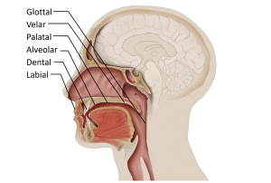
So, to sum it up, the three mechanisms that we use to produce speech are:
- Respiration (At the lungs): Energy comes from the air supplied by the lungs.
- Phonation (At the larynx): The vocal folds produce sound at the larynx.
- Articulation (In the mouth): The south is filtered, or shaped, by the articulators.
Wikipedia, Larynx URL: https://commons.wikimedia.org/wiki/File:Illu_larynx.jpg License: Public Domain
Introduction to Sensation and Perception Copyright © 2022 by Students of PSY 3031 and Edited by Dr. Cheryl Olman is licensed under a Creative Commons Attribution 4.0 International License , except where otherwise noted.
Share This Book
Want to create or adapt books like this? Learn more about how Pressbooks supports open publishing practices.
9.2 The Standard Model of Speech Production
Speech production falls into three broad areas: conceptualization, formulation and articulation (Levelt, 1989). In conceptualization , we determine what to say. This is sometimes known as message-level processing. Then we need to formulate the concepts into linguistic forms. Formulation takes conceptual entities as input and connects them with the relevant words associated with them to build a syntactic, morphological, and phonological structure. This structure is phonetically encoded and articulated , resulting in speech.
During conceptualization, we develop an intention and select relevant information from the internal (memory) or external (stimuli) environment to create an utterance. Very little is known about this level as it is pre-verbal. Levelt (1989) divided this stage into microplanning and macroplanning. Macroplanning is thought to be the elaboration of a communication goal into subgoals and connecting them with the relevant information. Microplanning assigns the correct shape to these pieces of information and deciding on the focus of the utterance.
Formulation is divided into lexicalization and syntactic planning . In lexicalization, we select the relevant word-forms and in syntactic planning we put these together into a sentence. In talking about word-forms, we need to consider the idea of lemmas . This is the basic abstract conceptual form which is the basis for other derivations. For example, break can be considered a lemma which is the basis for other forms such as break , breaks , broke , broken and breaking . Lemma retrieval used a conceptual structure to retrieve a lemma that makes syntactic properties available for encoding (Kempen & Hoenkamp, 1987). This can specify the parameters such as number, tense, and gender. During word-form encoding, the information connected to lemmas is used to access the morphemes and phonemes linked to the word. The reason these two processing levels, lemma retrieval and word-form encoding, are assumed to exist comes from speech errors where words exchange within the same syntactic categories. For example, nouns exchange with nouns and verbs with verbs from different phrases. Bierwisch (1970), Garrett (1975, 1980) and Nooteboom (1967) provide some examples:
- “… I left my briefcase in the cigar ”
- “What we want to do is train its tongue to move the cat ”
- “We completely forgot to add the list to the roof ”
- “As you reap , Roger, so shall you sow ”
We see here that not only are the exchange of words within syntactic categories, the function words associated with the exchanges appear to be added after the exchange (as in ‘its’ before ‘tongue’ and ‘the’ before ‘cat’). In contrast to entire words (which exchange across different phrases), segment exchanges usually occur within the same phrase and do not make any reference to syntactic categories. Garrett (1988) provides an example in “she is a real r ack p at” instead of “she is a real pack rat.” In such errors, the segments involved in the error often share phonetic similarities or share the same syllable position (Dell, 1984). This suggests that these segments must be operating within some frame such as syllable structure. To state this in broader terms, word exchanges are assumed to occur during lemma retrieval, and segment exchanges occur during word-form encoding.
Putting these basic elements together, Meyer (2000) introduced the ‘Standard Model of Word-form Encoding’ (see Figure 9.2) as a summation of previously proposed speech production models (Dell, 1986; Levelt et al., 1999; Shattuck-Huffnagel, 1979, 1983; Fromkin, 1971, 1973; Garrett, 1975, 1980). The model is not complete in itself but a way for understanding the various levels assumed by most psycholinguistic models. The model represents levels for morphemes, segments, and phonetic representations.

Morpheme Level
We have already seen (in Chapter 3 ) that morphemes are the smallest units of meaning. A word can be made up on one or more morphemes. Speech errors involving morphemes effect the lemma level or the wordform level (Dell, 1986) as in:
- “how many pies does it take to make an apple ?” (Garrett, 1988)
- “so the apple has less trees ” (Garrett, 2001)
- “I’d hear one if I knew it” (Garrett, 1980)
- “… slice ly thinn ed” (Stemberger, 1985)
In the first, we see that the morpheme that indicates the plural number has remained in place while the morpheme for ‘apple’ and ‘pie’ exchanged. This is also seen in the last example. This suggests that the exchange occurred after the parameters for number were set indicating that lemmas can switch independent of their morphological and phonological representations (which occur further down in speech production).
Segment Level
While speech production models differ in their organisation and storage of segments, we will assume thay segments have to be retrieved at some level of speech production. Between 60-90% of all speech errors tend to involve segments (Boomer & Laver, 1968; Fromkin, 1971; Nooteboom, 1969; Shattuck-Hufnagel, 1983). However, 10-30% of all speech errors also involve segment sequences (Stemberger, 1983; Shattuck-Hufnagel, 1983). Reaction time experiments have also been employed to justify this level. Roeloffs (1999) asked participants to learn a set of word pairs followed by the first word in the pair being presented as a prompt to produce the second word. These test blocks were presented as either homogeneous or heterogenous phonological forms. In the homogenous blocks there were shared onsets or the segments differed only in voicing. In the heterogenous blocks the initial segments contrasted in voicing and place of articulation. He found that there were priming effects in homogenous blocks when the targets shared an initial segment but not when all but one feature was shared suggesting that whole phonological segments are represented at some level rather than distinctive features.
Phonetic Level
The segmental level we just discussed is based on phonemes. The standard understanding of speech is that there must be a phonetic level that represents the actual articulated speech as opposed to the stored representations of sound. We have already discussed this in Chapter 2 and will expand here. For example, in English, there are two realizations of unvoiced stops. One form is unaspirated /p/, /k/, and /t/ and the other is aspirated [ph], [kh], and [th]. This can be seen in the words pit [phɪt] and lip [lɪp] where syllable-initial stops are aspirated as a rule. The pronunciation of pit as *[pɪt] doesn’t change the meaning but will sound odd to a native speaker. This shows that /p/ has one phonemic value but two phonetic values: [p] and [ph]. This can be understood as going from an abstract level to a concrete level developing as speech production occurs. Having familiarized ourselves with the basic levels of speech production, we can now go on to see how they are realized in actual speech production models.
Image descriptions
Figure 9.2 The Standard Model of Speech Production
The Standard Model of Word-form Encoding as described by Meyer (2000), illustrating five level of summation of conceptualization, lemma, morphemes, phonemes, and phonetic levels, using the example word “tiger”. From top to bottom, the levels are:
- Semantic level: the conceptualization of “tiger” with an image of a tiger.
- Lemma level: select the lemma of the word “tiger”.
- Morpheme level: morphological encoding of the word tiger, t, i, g, e, r.
- Phoneme level: phonological encoding of each morpheme in the word “tiger”.
- Phonetic kevel: syllabification of the phonemes in the word “tiger”.
[Return to place in text (Figure 9.2)]
Media Attributions
- Figure 9.2 The Standard Model of Speech Production by Dinesh Ramoo, the author, is licensed under a CC BY 4.0 licence .
The process of forming a concept or idea.
The creation of the word form during speech production.
The formation of speech.
The process of developing a word for production.
The planning of word order in a sentence.
The form of a word as it is presented at the head of an entry in a dictionary.
Psychology of Language Copyright © 2021 by Dinesh Ramoo is licensed under a Creative Commons Attribution 4.0 International License , except where otherwise noted.
Share This Book
Speech production and acoustic properties
2.2. speech production and acoustic properties #, 2.2.1. physiological speech production #, 2.2.1.1. overview #.
When a person has the urge or intention to speak, her or his brain forms a sentence with the intended meaning and maps the sequence of words into physiological movements required to produce the corresponding sequence of speech sounds. The neural part of speech production is not discussed further here.
The physical activity begins by contracting the lungs, pushing out air from the lungs, through the throat, oral and nasal cavities. Airflow in itself is not audible as a sound - sound is an oscillation in air pressure. To obtain a sound, we therefore need to obstruct airflow to obtain an oscillation or turbulence. Oscillations are primarily produced when the vocal folds are tensioned appropriately. This produces voiced sounds and is perhaps the most characteristic property of speech signals. Oscillations can also be produced by other parts of the speech production organs, such as letting the tongue oscillate against the teeth in a rolling /r/, or by letting the uvula oscillate in the airflow, known as the uvular trill (viz. something like a guttural /r/). Such trills, both with the tongue and the uvula, should however not be confused with voiced sounds, which are always generated by oscillations in the vocal folds. Sounds without oscillations in the vocal folds are known as unvoiced sounds.
Most typical unvoiced sounds are caused by turbulences produced by static constrictions of airflow in any part of the air spaces above the vocal folds (viz. larynx, pharynx and oral or nasal cavities). For example, by letting the tongue rest close to the teeth, we obtain the consonant /s/, and by stopping and releasing airflow by closing and opening the lips, we obtain the consonant /p/. A further particular class of phonemes are nasal consonants, where airflow through the mouth is stopped entirely or partially, such that a majority of the air flows through the nose.
2.2.1.2. The vocal folds #
The vocal folds, also known as vocal cords, are located in the throat and oscillate to produce voiced sounds. The opening between the vocal folds (the empty space between the vocal folds) is known as the glottis . Correspondingly, the airspace between the vocal folds and the lungs is known as the subglottal area.
When the pressure below the glottis, known as the subglottal pressure increases, it pushes open the vocal folds. When open, air rushes through the vocal folds. The return movement, again closing the vocal folds is mainly caused by the Venturi effect , which causes a drop in air pressure between the vocal folds when air is flowing through them. As the vocal folds are closing, they will eventually clash together. This sudden stop of airflow is the largest acoustic event in the vocal folds and is known as the glottal excitation .
In terms of airflow, the effect is that during the closed phase (when the vocal folds are closed), there is no airflow. At the beginning of the open phase (when the vocal fold are open), air starts to flow through the glottis and obviously, with the closing of the vocal folds also air flow is decreasing. However, due to the momentum of air itself, the movement of air occurs slightly after the vocal folds. In other words, there is a phase-difference between vocal folds movement and glottal airflow waveform.
The frequency of vocal folds oscillation is dependent on three main components; amount of lengthwise tension in the vocal folds, pressure differential above and below the vocal folds, as well as length and mass of the vocal folds. Pressure and tension can be intentionally changed to cause a change in frequency. The length and mass of the vocal folds are in turn correlated with overall body size of the speaker, which explains the fact that children and females have on average a higher pitch than male speakers.
Note that the frequency of the vocal folds refers to the actual physical phenomenon, whereas pitch refers to the perception of frequency. There are many cases where these two may differ, for example, resonances in the vocal tract can emphasise harmonics of the fundamental frequency such that the harmonics are louder than the fundamental, and such that we perceive one of the harmonics as the fundamental. The perceived pitch is then the frequency of the harmonic instead of the fundamental.
2.2.1.3. The vocal tract #
The vocal tract, including the larynx, pharynx and oral cavities, have a great effect on the timbre of the sound. Namely, the shape of the vocal tract determines the resonances and anti-resonances of the acoustic space, which boost and attenuate different frequencies of the sound. The shape is determined by a multitude of components, in particular by the position of the jaw, lips and tongue. The resonances are easily modified by the speaker and perceived by the listener, and they can thus be used in communication to convey information. Specifically, the acoustic features which differentiate vowels from each other are the frequencies of the resonances in the vocal tract, corresponding to specific places of articulation primarily in terms of tongue position. Since the air can flow relatively unobstructed, vowel sounds tend to have high energy and loudness compared to consonants .
In consonant sounds, there is a partial or full obstruction at some part of the vocal tract. For instance, fricative consonants are characterized by a narrow gap between the tongue and front/top of the mouth, leading to hiss-like turbulent air flow. In plosives, the airflow in the vocal tract is fully temporarily obstructed. As an example, bilabial plosives are characterized by temporary closure of the lips, which leads to accumulation of air pressure in the vocal tract due to sustained lung pressure. When the lips are opened, the accumulated air is released together with a short burst sound (plosion) that has impulse- and noise-like characteristics. Similarly to vowels, the place of the obstruction in the mouth (i.e., place of articulation) will affect the acoustic characteristics of the consonant sound by modifying the acoustic characteristics of the vocal tract. In addition, manner of articulation is used to characterize different consonant sounds, as there are several ways to produce speech while the position of the primary obstruction can remain the same (e.g., short taps and flaps , repeated trills, or already mentioned narrow constrictions for fricatives ).
In terms of vocal tract shape, a special class of consonants are the nasals , which are produced with velum (a soft structure at the back top of the oral cavity) open, thereby allowing air to flow to the nasal cavity . When the velum is open, the vocal tract can be viewed as a shared tube from the larynx to the back of the mouth, after which the tract is divided into two parallel branches consisting of the oral and nasal cavities. Coupling of the nasal cavity to the vocal tract has a pronounced impact on the resonances and anti-resonance of the tract. This is commonly perceived as nasalization of speech sounds by listeners.
Side-view of the speech production organs.

By BruceBlaus. When using this image in external sources it can be cited as: Blausen.com staff (2014). “Medical gallery of Blausen Medical 2014”. WikiJournal of Medicine 1 (2). DOI:10.15347/wjm/2014.010. ISSN 2002-4436. - Own work, CC BY 3.0, https://commons.wikimedia.org/w/index.php?curid=29294598
Vocal folds as seen from above.

The motion of vocal folds seen from the front (or back).
Organs in the mouth.

The four images above are from Wikipedia.
2.2.2. Acoustic properties of speech signals #
The most important acoustic features of a speech signal are (roughly speaking)
The resonance of the vocal tract , especially the two lowest resonances, known as the formants F1 and F2 (see figure below). The resonance structure can be easily examined by drawing an “ envelope” above the spectrum, that is, to draw a smooth line which goes just above the spectrum, as seen on the figure below. We thus obtain the spectral envelope , which characterizes the macro-shape of the spectrum of a speech signal, and which is often used to model speech signals.
The fundamental frequency of a speech signal or its absence carries a lot of information. Per definition, voiced and unvoiced phonemes, respectively, are those with or without an oscillation in the vocal folds. Due to its prominence, we categorize phonemes according to whether they are voiced or unvoiced. The airflow which passes through the oscillating vocal folds will generally have a waveform which resembles a half-wave rectified sinusoid . That is, airflow is zero when the vocal folds are closed (closed phase) and during the open time (open phase) the waveform resembles (somewhat) the shape of the upper part of a sinusoid. The spectrum of this waveform will therefore have the structure of a harmonic signal, that is, the spectrum will have peaks at the fundamental frequency and its integer multiples (see figure below). In most languages, pitch does not differentiate between phonemes. However, in languages that are known as tonal languages, the shape of the pitch contour over time does bear semantic meaning (see Wikipedia:Tone (linguistics) for a nice sound sample). Pitch contours are however often used to encode emphasis in a sentence. Roughly speaking, exerting more physical effort on a phoneme raises its pitch and intensity, and that is usually interpreted as emphasis, that is, the word (or phoneme) with emphasis is more important than other words (or phonemes) in a sentence.
Signal amplitude or intensity over time is another important characteristic and in its most crude form can be the difference between speech and silence (see also Voice activity detection (VAD) ). Furthermore, there are phonemes characterized by their temporal structure; in particular, stop and plosive-consonants , where airflow is stopped and subsequently released (e.g. /p/, /t/ and /k/). While the stop-part is not prominently audible, it is the contrast of a silence before a burst of energy which characterizes these consonants.

The waveform of a sentence of speech, illustrating variations in amplitude and intensity.

2.2.3. Physiological modelling #
2.2.3.1. vocal tract #.
Vowels are central to spoken communication, and vowels are determined by the shape of the vocal tract. Modelling the vocal tract is therefore of particular interest.
2.2.3.1.1. Simple models #
The vocal tract is essentially a tube of varying length. It has a 90-degree bend, where the throat turns into the mouth, but the acoustic effect of that bend is minor and can be ignored in simple models. The tube has two pathways, through the oral and nasal cavities. The acoustic effect of the oral cavity dominates the output signal such that, roughly speaking, the oral cavity generates resonances to the output sound, while the nasal cavities contributes mainly anti-resonances (dips or valleys) to the spectral envelope. Presence of energy is perceptually more important than absence of energy and anti-resonances can therefore be ignored in simple models.
A very simple model is thus a straight cylindrical tube sub-divided into constant radius segments of equal length (see illustration below). If we further assume that the tube-segments are lossless, then this tube is analytically equivalent with a linear predictor . This is a fantastic simplification in the sense that from a physiologically motivated model we obtain a analytically reasonable model whose parameters we can readily estimate from observed signals. In fact, the temporal correlation of speech signals can be very efficiently modelled with linear predictors. It offers a very attractive connection between physiological and signal modelling. Unfortunately, it is not entirely accurate.
Though speech signals are very efficiently modelled by linear predictors, and linear predictors are analytically equivalent with tube-models, linear predictors estimated from sound signals need not correspond to the tube which generated the sound . The mismatch in the shape of estimated and real tubes is due to two primary reasons;
Estimation of linear predictive coefficients assumes that the excitation, viz. the glottal excitation, is uncorrelated (white noise). This is certainly an incorrect assumption. Though the periodic structure of the glottal excitation does not much bias linear predictors, glottal excitations are also dominated by low-frequency components which will bias the linear predictor. The linear predictor cannot make a distinction between features of the glottal excitation and contributions of the vocal tract, but model both indiscriminately. We also do not know the precise contribution of the glottal excitation such that it is hard to compensate for it.
The analytical relationship between coefficients of the linear predictor and the radii of the tube-model segments is highly non-linear and sensitive to estimation errors. Small errors in predictor parameters can have large consequences in the shape of the tube model.
Still, since linear predictors are efficient for modelling speech, they are useful in speech modelling even if the connection to tube-modelling is sensitive to errors. Linear prediction is particularly attractive because it gives computationally efficient algorithms.
2.2.3.1.2. Advanced models #
When more accurate modelling of the vocal tract is required, we have to re-evaluate our assumptions. With digital waveguides we can readily formulate models which incorporate a second pathway corresponding to the nasal tract. A starting point for such models is linear prediction, written as a delay-line with reflections corresponding to the interfaces between tube-segments. The nasal tract can then be introduced by adding a second delay line. Such models are computationally efficient in synthesis of sounds, but estimating their parameters from real sounds can be difficult.
Stepping up the accuracy, we then already go into full-blown physical modelling such as finite-element methods (FEM). Here, for example, the air-volume of the vocal tract can be split into small interacting elements governed by fluid dynamics . The more dense the mesh of the elements is, the more accurately the model corresponds to physical reality. Measuring and modelling the vocal tract with this method is involved and an art form of its own .

Illustration of a vocal-tract tube-model consisting of piece-wise constant-radius tube-segments.
2.2.3.2. Glottal activity #
As characterization of the glottal flow, we define events of a single glottal period as follows (illustrated in the figure below):
Opening and closing time (or instant), are the points in time where respectively, glottal folds open and close, and where glottal flow starts and ends.
Open and closed phase , are the periods during which the glottis is open and closed, respectively.
The length of time when glottis is open and closed are, respectively, known as open time (OT) and closed time (CT) . Consequently, the period length is \(T=OT+CT\) .
Opening and closing phases are the portions of the open phase, when the glottis is opening and closing, respectively.
The steepness of the closing phase is related to the “agressiveness” of the pulse, that is, it relates to the tension of glottal folds and is characterized by the (negative) peak of the glottal flow derivative .
All parameters describing a length in time are often further normalized by the period length \(t\) .
Like modelling of the vocal tract, also in modelling glottal activity, there is a range of models of different complexity:
Maximum-phase linear prediction ; The most significant event in a single glottal flow pulse is its closing instant; the preceding waveform is smooth but the closing event is abrupt. The waveform can thus be interpreted as the impulse response of an IIR filter but turned backwards, which also known as the impulse response of a maximum-phase linear predictor (the figure on the right was generated with this method). The beauty of this method is that it is similar to vocal tract modelling with linear prediction, such that we are already familiar with the method and computational complexity is simple. Observe, however, that maximum-phase filters are by definition unstable (not realizable), but we have to always process the signal backwards, which complicates systems design.
The Liljencrantz-Fant (LF) -model is a classical model of the glottal flow, the original form of which is a function of four parameters ( defined in article ). It is very useful and influential because it parametrizes the flow with a low number of easily understandable parameters. The compromise is that the parameters are not easily estimated from real signals and that it is based on anecdotal evidence of glottal flow shapes and if it were presented today, to be widely accepted, we would require more evidence to support it.
Mass-spring systems ; the opposing glottal folds can be modelled as simple point-masses connected with damped springs to fixed points. When subjected to the Venturi-forces generated by the airflow, these masses can be brought to oscillate like the vocal folds. Such models are attractive because, again, their parameters have physical interpretations, but since their parameters are difficult to estimate from real-world data and they oscillate only a limited range of the parameters, their usefulness in practical applications is limited.
Finite-element methods (FEM) are again the ultimate method for accurate analysis, suitable for example in medical analysis, yet the computational complexity is prohibitively large for consumer applications.

Illustration of a glottal flow pulse, its derivative and a sequence of glottal flow pulses (corresponding sound below).
2.2.3.3. Lip radiation #
Having travelled through the vocal tract, air exits primarily through the mouth and in some extent through the nose. In leaving this tube, it enters the free field where airflow in has little effect. Recall that sounds are, instead, variations in air pressure. At the transition from the tube to the free field, variations in air flow become variations in air pressure.
The physics of this phenomenon are governed by fluid dynamics , an advanced topic, but heuristically we can imagine that variations air pressure is related to variations in airflow. Thus if we take the derivative of the airflow, we get an approximation of its effect on air pressure
where \(t\) is time.
Often we deal with signals sampled at time indices \(n\) , where the derivative can be further approximated by the first difference
where \(g>0\) is a scalar gain coefficient.
Overview of Speech Production and Speech Mechanism
Overview of Speech Production and Speech Mechanism: Communication is a fundamental aspect of human interaction, and speech production is at the heart of this process. Behind every spoken word lies a series of intricate steps that allow us to convey our thoughts and ideas effectively. Speech production involves three essential levels: conceptualization, formulation, and articulation. In this article, we will explore each level and understand how they contribute to the seamless flow of communication.
Overview of Speech Production
Speech Production deals in 3 levels:
Conceptualization
Formulation , articulation .
Speech production is a remarkable process that involves multiple intricate levels. From the initial conceptualization of ideas to their formulation into linguistic forms and the precise articulation of sounds, each stage plays a vital role in effective communication. Understanding these levels helps us appreciate the complexity of human speech and the incredible coordination between the brain and the vocal tract. By honing our speech production skills, we can become more effective communicators and forge stronger connections with others.

Steps of Speech Production
Conceptualization is the first level of speech production, where ideas and thoughts are born in the mind. At this stage, a person identifies the message they want to convey, decides on the key points, and organizes the information in a coherent manner. This process is highly cognitive and involves accessing knowledge, memories, and emotions related to the topic.
During conceptualization, the brain’s language centers, such as the Broca’s area and Wernicke’s area, play a crucial role. The Broca’s area is involved in the planning and sequencing of speech, while the Wernicke’s area is responsible for understanding and accessing linguistic information.
For example, when preparing to give a presentation, the conceptualization phase involves structuring the content logically, identifying the main ideas, and determining the tone and purpose of the speech.
The formulation stage follows conceptualization and involves transforming abstract thoughts and ideas into linguistic forms. In this stage, the brain converts the intended message into grammatically correct sentences and phrases. The formulation process requires selecting appropriate words, arranging them in a meaningful sequence, and applying the rules of grammar and syntax.
At the formulation level, the brain engages the motor cortex and the areas responsible for language production. These regions work together to plan the motor movements required for speech.
During formulation, individuals may face challenges, such as word-finding difficulties or grammatical errors. However, with practice and language exposure, these difficulties can be minimized.
Continuing with the previous example of a presentation, during the formulation phase, the speaker translates the organized ideas into spoken language, ensuring that the sentences are clear and coherent.
Articulation is the final level of speech production, where the formulated linguistic message is physically produced and delivered. This stage involves the precise coordination of the articulatory organs, such as the tongue, lips, jaw, and vocal cords, to create the specific sounds and speech patterns of the chosen language.
Smooth and accurate articulation is essential for clear communication. Proper articulation ensures that speech sounds are recognizable and intelligible to the listener. Articulation difficulties can lead to mispronunciations or speech disorders , impacting effective communication.
In the articulation phase, the motor cortex sends signals to the speech muscles, guiding their movements to produce the intended sounds. The brain continuously monitors and adjusts these movements to maintain the fluency of speech.
For instance, during the presentation, the speaker’s articulation comes into play as they deliver each sentence, ensuring that their words are pronounced correctly and clearly.
Overview of Speech Mechanism

Speech Sub-system
The speech mechanism is a complex and intricate process that enables us to produce and comprehend speech. The speech mechanism involves a coordinated effort of speech subsystems working together seamlessly. Speech Mechanism is done by 5 Sub-systems:
- Respiratory System
Phonatory System
- Resonatory System
- Articulatory System
Regulatory System
I. Respiratory System
Respiration: The Foundation of Speech
Speech begins with respiration, where the lungs provide the necessary airflow. The diaphragm and intercostal muscles play a crucial role in controlling the breath, facilitating the production of speech sounds.
II. Phonatory System
Phonation: Generating the Sound Source
Phonation refers to the production of sound by the vocal cords in the larynx. As air from the lungs passes through the vocal cords, they vibrate, creating the fundamental frequency of speech sounds.
Phonation, in simple terms, refers to the production of sound through the vibration of the vocal folds in the larynx. When air from the lungs passes through the vocal folds, they rapidly open and close, generating vibrations that produce sound waves. These sound waves then resonate in the vocal tract, shaping them into distinct speech sounds.
The Importance of Phonation in Speech Production
Phonation is a fundamental aspect of speech production as it forms the basis for vocalization. The process allows us to articulate various speech sounds, control pitch, and modulate our voices to convey emotions and meaning effectively.
Mechanism of Phonation

Vocal Fold Structure
To understand phonation better, we must examine the structure of the vocal folds. The vocal folds, also known as vocal cords, are situated in the larynx (voice box) and are composed of elastic tissues. They are divided into two pairs, with the true vocal folds responsible for phonation.
The Process of Phonation
The process of phonation involves a series of coordinated movements. When we exhale, air is expelled from the lungs, causing the vocal folds to close partially. The buildup of air pressure beneath the closed vocal folds causes them to be pushed open, releasing a burst of air. As the air escapes, the vocal folds quickly close again, repeating the cycle of vibrations, which results in a continuous sound stream during speech.
III. Resonatory System
Resonance: Amplifying the Sound
The sound produced in the larynx travels through the pharynx, oral cavity, and nasal cavity, where resonance occurs. This amplification process adds richness and depth to the speech sounds.
IV. Articulatory System
Articulation: Shaping Speech Sounds
Articulation involves the precise movements of the tongue, lips, jaw, and soft palate to shape the sound into recognizable speech sounds or phonemes.
When we speak, our brain sends signals to the muscles responsible for controlling these speech organs, guiding them to produce different articulatory configurations that result in distinct sounds. For example, to form the sound of the letter “t,” the tongue makes contact with the alveolar ridge (the ridge behind the upper front teeth), momentarily blocking the airflow before releasing it to create the characteristic “t” sound.
The articulation process is highly complex and allows us to produce a vast array of speech sounds, enabling effective communication. Different languages use different sets of speech sounds, and variations in articulation lead to various accents and dialects.
Efficient articulation is essential for clear and intelligible speech, and any impairment or deviation in the articulatory process can result in speech disorders or difficulties. Speech therapists often work with individuals who have articulation problems to help them improve their speech and communication skills. Understanding the mechanisms of articulation is crucial in studying linguistics, phonetics, and the science of speech production.
Articulators are the organs and structures within the vocal tract that are involved in shaping the airflow to produce specific sounds. Here are some of the main articulators and the sounds they help create:

- The tongue is one of the most versatile articulators and plays a significant role in shaping speech sounds.
- It can move forward and backward, up and down, and touch various parts of the mouth to produce different sounds.
- For example, the tip of the tongue is involved in producing sounds like “t,” “d,” “n,” and “l,” while the back of the tongue is used for sounds like “k,” “g,” and “ng.”
- The lips are essential for producing labial sounds, which involve the use of the lips to shape the airflow.
- Sounds like “p,” “b,” “m,” “f,” and “v” are all labial sounds, where the lips either close or come close together during articulation.
- The teeth are involved in producing sounds like “th” as in “think” and “this.”
- In these sounds, the tip of the tongue is placed against the upper front teeth, creating a unique airflow pattern.
Alveolar Ridge:
- The alveolar ridge is a small ridge just behind the upper front teeth.
- Sounds like “t,” “d,” “s,” “z,” “n,” and “l” involve the tongue making contact with or near the alveolar ridge.
- The palate, also known as the roof of the mouth, plays a role in producing sounds like “sh” and “ch.”
- These sounds, known as postalveolar or palato-alveolar sounds, involve the tongue articulating against the area just behind the alveolar ridge.
Velum (Soft Palate):
- The velum is the soft part at the back of the mouth.
- It is raised to close off the nasal cavity during the production of non-nasal sounds like “p,” “b,” “t,” and “d” and lowered to allow airflow through the nose for nasal sounds like “m,” “n,” and “ng.”
- The glottis is the space between the vocal cords in the larynx.
- It plays a role in producing sounds like “h,” where the vocal cords remain open, allowing the airflow to pass through without obstruction.
By combining the movements and positions of these articulators, we can produce the vast range of speech sounds used in different languages around the world. Understanding the role of articulators is fundamental to the study of phonetics and speech production .
V. Regulatory system

Regulation: The Role of the Brain and Nervous System
The brain plays a pivotal role in controlling and coordinating the speech mechanism.
Broca’s Area: The Seat of Speech Production
Located in the left frontal lobe, Broca’s area is responsible for speech production and motor planning for speech movements.
Wernicke’s Area: Understanding Spoken Language
Found in the left temporal lobe, Wernicke’s area is crucial for understanding spoken language and processing its meaning.
Arcuate Fasciculus: Connecting Broca’s and Wernicke’s Areas
The arcuate fasciculus is a bundle of nerve fibers that connects Broca’s and Wernicke’s areas, facilitating communication between speech production and comprehension centers.
Motor Cortex: Executing Speech Movements
The motor cortex controls the muscles involved in speech production, translating neural signals into precise motor movements.
References :
- Speech Science Primer (Sixth Edition) Lawrence J. Raphael, Gloria J. Borden, Katherine S. Harris [Book]
- Manual on Developing Communication Skill in Mentally Retarded Persons T.A. Subba Rao [Book]
- SPEECH CORRECTION An Introduction to Speech Pathology and Audiology 9th Edition Charles Van Riper [Book]
You are reading about:
Share this:.
- Click to share on Twitter (Opens in new window)
- Click to share on Facebook (Opens in new window)
- Click to share on LinkedIn (Opens in new window)
- Click to share on Telegram (Opens in new window)
- Click to share on WhatsApp (Opens in new window)
- Click to print (Opens in new window)

Written by BASLPCOURSE.COM
July 26, 2023, baslp 1st semester anatomy and physiology of speech and hearing notes | baslp 1st semester anatomy and physiology of speech and hearing unit 3 notes | baslp 1st semester communication science notes | baslp 1st semester communication science unit 2 notes | baslp 1st semester linguistics and phonetics notes | baslp 1st semester linguistics and phonetics unit 2 notes | baslp 1st semester notes | baslp 3rd semester notes | baslp 3rd semester speech sound disorders notes | baslp 3rd semester speech sound disorders unit 2 notes | baslp 4th semester motor speech disorders in children notes | baslp 4th semester motor speech disorders in children unit 1 notes | baslp 4th semester notes | baslp notes | blog | speech and language pathology, 0comment(s), follow us on.
For more updates follow us on Facebook, Twitter, Instagram, Youtube and Linkedin
You may also like….

Types of Earmolds for Hearing Aid – Skeleton | Custom
Jan 18, 2024
Types of Earmolds for Hearing Aid - Skeleton | Custom: The realm of hearing aids is a diverse landscape with a myriad...

Procedure for Selecting Earmold and Earshell
Jan 17, 2024
Procedure for Selecting Earmold and Earshell: When it comes to optimizing the acoustic performance of hearing aids,...

Ear Impression Techniques for Earmolds and Earshells
Jan 16, 2024
Ear Impression Techniques for Earmolds and Earshells: In the realm of audiology and hearing aid fabrication, the Ear...
If you have any Suggestion or Question Please Leave a Reply Cancel reply
Want to create or adapt books like this? Learn more about how Pressbooks supports open publishing practices.
9.1 Evidence for Speech Production
Dinesh Ramoo
The evidence used by psycholinguistics in understanding speech production can be varied and interesting. These include speech errors, reaction time experiments, neuroimaging, computational modelling, and analysis of patients with language disorders. Until recently, the most prominent set of evidence for understanding how we speak came from speech errors . These are spontaneous mistakes we sometimes make in casual speech. Ordinary speech is far from perfect and we often notice how we slip up. These slips of the tongue can be transcribed and analyzed for broad patterns. The most common method is to collect a large corpus of speech errors by recording all the errors one comes across in daily life.
Perhaps the most famous example of this type of analysis are what are termed ‘ Freudian slips .’ Freud (1901-1975) proposed that slips of the tongue were a way to understand repressed thoughts. According to his theories about the subconscious, certain thoughts may be too uncomfortable to be processed by the conscious mind and can be repressed. However, sometimes these unconscious thoughts may surface in dreams and slips of the tongue. Even before Freud, Meringer and Mayer (1895) analysed slips of the tongue (although not in terms of psychoanalysis).
Speech errors can be categorized into a number of subsets in terms of the linguistic units or mechanisms involved. Linguistic units involved in speech errors could be phonemes, syllables, morphemes, words or phrases. The mechanisms of the errors can involve the deletion, substitution, insertion, or blending of these units in some way. Fromkin (1971; 1973) argued that the fact that these errors involve some definable linguistic unit established their mental existence at some level in speech production. We will consider these in more detail in discussing the various stages of speech production.
| Error Type | Error | Target |
|---|---|---|
| Anticipation | eading list | Reading list |
| Perseveration | black oxes | black boxes |
| Exchange | at ack | pack rat |
| Substitution | s encil | stencil |
| Deletion | sippery | slippery |
| Insertion | s kool | school |
An error in the production of speech.
An unintentional speech error hypothesized by Sigmund Freud as indicating subconscious feelings.
9.1 Evidence for Speech Production Copyright © 2021 by Dinesh Ramoo is licensed under a Creative Commons Attribution-NonCommercial-ShareAlike 4.0 International License , except where otherwise noted.
Share This Book

Exploring the Wonders of Speech: What is Speech and How Does it Work?
Speech is an intricate and remarkable aspect of human communication. It’s the primary means by which we express our thoughts, share our emotions, and connect with others. But what exactly is speech, and how does it work? In this blog, we’ll delve into the fascinating world of speech , exploring its components, functions, and the science behind this remarkable ability.
Understanding Speech: The Basics
Speech is the vocalized form of human communication. It involves the production and articulation of sounds to convey meaning and thoughts. This intricate process combines physiological, cognitive, and linguistic elements to create a rich tapestry of communication.
Components of Speech
- Phonemes: Phonemes are the smallest distinct units of sound in a language. Different languages have different sets of phonemes, and combining these phonemes in various ways forms words and sentences.
- Articulation: Articulation refers to the movement of the vocal organs (such as the lips, tongue, and vocal cords) to produce specific sounds. The precise coordination of these movements allows us to create a diverse range of sounds.
- Prosody: Prosody encompasses the rhythm, intonation, and stress patterns in speech. It adds emotional nuances and conveys intentions, like whether a statement is a question or a declaration.
The Science Behind Speech Production
Speech production involves a complex interplay of the brain, vocal apparatus, and linguistic knowledge. Here’s a simplified breakdown of the process:
- Brain Activation: The brain’s language centers, including Broca’s area and Wernicke’s area, play crucial roles in speech production and comprehension. These areas coordinate the planning and execution of speech.
- Speech Planning: The brain formulates the intended message into linguistic units (words and phrases). It then sends signals to the motor cortex, which controls the movements of the vocal organs.
- Vocal Cord Vibrations: As air from the lungs passes through the vocal cords, they vibrate. This vibration generates sound waves, which are then shaped into specific sounds by manipulating the vocal organs.
- Articulation: The tongue, lips, teeth, and other vocal organs work together to modify the airflow and shape the sound waves. This process results in the production of different phonemes.
- Auditory Feedback: The brain constantly monitors the sounds being produced and compares them to the intended speech. This feedback loop allows for real-time adjustments to pronunciation.
Functions of Speech
- Communication: The primary function of speech is to convey information, thoughts, feelings, and intentions to others.
- Social Interaction: Speech plays a pivotal role in social interactions, enabling connections, friendships, and cooperation among individuals.
- Cultural Transmission: Through speech, cultures pass down traditions, stories, and knowledge from one generation to the next.
- Learning and Education: Speech is essential for learning languages, acquiring new information, and participating in educational activities.
Speech is a marvel of human evolution, blending cognitive abilities, linguistic knowledge, and intricate motor coordination. It allows us to connect, express, and understand each other in ways that written language cannot replicate. Understanding the components and science behind speech sheds light on the complexity of this everyday phenomenon and deepens our appreciation for the power of communication .
Recent Posts

- Unlocking Speech through Pediatric Occupational Therapy for Kids - June 26, 2024
- News of the month for March 2024 - April 16, 2024
- News of the month for Jan 2024 - January 29, 2024
Leave a Comment
(0 Comments)
Cancel reply

Your email address will not be published. Required fields are marked *
Save my name, email, and website in this browser for the next time I comment.
- Mental Health
- Multilingual
- Occupational Therapy
- Speech Delay
- Speech Therapy
- Success Stories
- Unlocking Speech through Pediatric Occupational Therapy for Kids June 26, 2024
- News of the month for March 2024 April 16, 2024
- News of the month for Jan 2024 January 29, 2024
- Shining a Light on the Unseen: The Importance of Syndrome Awareness January 23, 2024
- Celebrating Excellence: Pratiksha Gupta Wins SABLA NARI Award for Best Speech Language Therapist and Audiologist 2023 January 19, 2024
Don't miss our one of its kind SPEAK EASY PROGRAM for stuttering management. Chat with us to know more! Dismiss
- Guest Posts
- Press Releases
- Journal Articles
- Supplemental Content
- Guest Podcasts
Select Page
4 Stages of Speech Production

Humans produce speech on a daily basis. People are social creatures and are always talking to one another. Whether it is through social media, live conversation, texting, chat, or otherwise, we are always producing some form of speech. We produce this speech without thought.
That is, without the thought of how we produce it. Of course, we think about what we are going to say and how to say it so that the other people will listen but we don’t think about what it is made of and how our mind and body actually product speech.
If you have been following my other language-related articles, then you will not be surprised to find out that there are four stages of speech production. It seems that those who classified this data did so in measures of fours and fives. There are…
Five Methods to Learn a Language
Four Ways to Assess Student Knowledge
Five Language Learning Strategies
Four Properties of Spoken Language
The list goes on! Now we have four stages of speech production. These are the processes by which humans produce speech. All of the ways that we come up with the words we say have been compiled into four stages. These stages are not consecutive like normal scientific stages. Instead, they are simply classified as such.
This means that they are not something you go through developmentally. Rather they are simply different ways in which you may produce speech. I’ll describe each one of them so you can learn and understand what they are and know how exactly you come up with everything you say.
Money To Invest… Stop Paying For Trades!
Stage 1 – Conceptualization
The first one is called the Conceptualization Stage. This is when a speaker spontaneously thinks of what he or she is going to say. It is an immediate reaction to external stimuli and is often based on prior knowledge of the particular subject. No premeditation goes into these words and they are all formulated based upon the speaker’s knowledge and experience at hand. It is spontaneous speech. Examples of this can range from answering questions to the immediate verbiage produced as a result of stubbing your toe.
Stage 2 – Formulation
The second stage is called the Formulation Stage. This is when the speaker thinks of the particular words that are going to express their thoughts. It occurs almost simultaneously with the conceptualization stage. However, this time the speaker thinks about the response before responding. The speaker is formulating his or her words and deciding how best to reply to the external stimuli. Where conceptualization is more of an instant and immediate response, formulation is a little delayed.
Stage 3 – Articulation
The third stage is the Articulation Stage. This is when the speaker physically says what he or she has thought of saying. This is a prepared speech or planned wordage. In addition, the words may have been rehearsed such as when someone practices a presentation or rehearses a lie.
It involves the training of physical actions of several motor speech organs such as the lungs, larynx, tongue, lips, and other vocal apparatuses. Of course, the first two stages also involve these organs, however, the articulation stage uses these organs multiple times for the same word patterns.
Stage 4 – Self-Monitoring
The fourth stage is called the Self-Monitoring Stage. This is when the speaker reflects on what he or she has said and makes an effort to correct any errors in his or her speech. Often times this is done in a rebuttal or last words argument.
In addition, it could also be done during a conversation when the speaker realizes that he or she slipped up. This is the action of reflecting on what you said and making sure that what you said is what you meant.
Real-Time Spell Check And Grammar Correction
There you have it. Those are the four stages of speech production. Think about this and start to notice each time you are in each stage. Of course, you won’t be able to consciously notice what stage you are in all of the time. However, once in a while it may be amusing for you to reflect on these stages and see how they coincide with the words you speak.
For more great information take a look at the supplemental content on this website and check out these great blog posts . In addition, feel free to connect with me on social media.
Enjoying This Content?
Consider donating to support spencer coffman, venmo paypal cashapp, related posts.

The Best Way To Use Facebook Ads To Increase Sales
December 25, 2017
7 Must-Have Apps For Business Owners
January 21, 2018

How To Check Your Recovery Rate After Working Out
November 13, 2017

Steemit Videos – Series on How to Succeed on Steemit
May 1, 2020
| ©1999 CCRMA, Stanford University. All Rights Reserved. , . | Look up a word, learn it forever.Speech production.
Sign up now (it’s free!)Whether you’re a teacher or a learner, vocabulary.com can put you or your class on the path to systematic vocabulary improvement.. Psycholinguistics/Development of Speech Production
IntroductionSpeech production is an important part of the way we communicate. We indicate intonation through stress and pitch while communicating our thoughts, ideas, requests or demands, and while maintaining grammatically correct sentences. However, we rarely consider how this ability develops. We know infants often begin producing one-word utterances, such as "mama," eventually move to two-word utterances, such as "gimme toy" and finally sound like an adult. However, the process itself involves development not only of the vocal sounds (phonology), but also semantics (meaning of words), morphology and syntax (rules and structure). How do children learn to this complex ability? Considering that an infant goes from an inability to speak to two-word utterances within 2 years, the accelerated development pattern is incredible and deserves some attention. When we ponder children's speech production development more closely, we begin to ask more questions. How does a child who says "tree" for "three" eventually learn to correct him/herself? How does a child know "nana" (banana) is the yellow,boat-shaped fruit he/she enjoys eating? Why does a child call all four-legged animals "horsie"? Why does this child say "I goed to the kitchen"? What causes a child to learn words such as "doggie" before "hand"? This chapter will address these questions and focus on the four areas of speech development mentioned: phonology, semantics, and morphology and syntax. Prelinguistic Speech DevelopmentThroughout infancy, vocalizations develop from automatic, reflexive vocalizations with no linguistic meaning to articulated words with meaning and intonation. In this section, we will examine the various stages an infant goes through while developing speech. In general, researchers seem to agree that as infants develop they increase their speech-like vocalizations and decrease their non-speech vocalizations (Nathani, Ertmer, & Stark) [1] . Many researchers (Oller, ; [2] Stark, as cited in Nathani, Ertmer, & Stark, 2006) [1] . Many researchers (Oller; [2] Stark, as cited in Nathani, Ertmer, & Stark,) [1] have documented this development and suggest growth through the following five stages: reflexive vocalizations, cooing and laughing, vocal play (expansion stage) , canonical babbling and finally, the integration stage. Stage 1: Reflexive Vocalization As newborns, infants make noises in responses to their environment and current needs. These reflexive vocalizations may consist of crying or vegetative sounds such as grunting, burping, sneezing, and coughing (Oller) [2] . Although it is often thought that infants of this age do not show evidence of linguistic abilities, a recent study has found that newborns’ cries follow the melody of their surrounding language input (Mampe, Friederici, Christophe, & Wermke) [3] . They discovered that the French newborns’ pattern was a rising contour, where the melody of the cry rose slowly and then quickly decreased. In comparison, the German newborns’ cry pattern rose quickly and slowly decreased. These patterns matched the intonation patterns that are found in each of the respective spoken languages. Their finding suggest that perhaps infants vocalizations are not exclusively reflexive and may contain patterns of their native language. Stage 2: Gooing, Cooing and LaughingBetween 2 and 4 months, infants begin to produce “cooing” and “gooing” to demonstrate their comfort states. These sounds may often take the form of vowel-like sounds such as “aah” or “oooh.” This stage is often associated with a happy infant as laughing and giggling begin and crying is reduced. Infants will also engage in more face-to-face interactions with their caregivers, smiling and attempting to make eye contact (Oller) [2] . Stage 3: Vocal PlayFrom 4 to 6 months, and infants will attempt to vary the sounds they can produce using their developing vocal apparatus. They show a desire to explore and develop new sounds which may include yells, squeals, growls and whispers(Oller) [2] . Face-to-face interactions are still important at this stage as it promotes development of conversation abililities. Beebe, Alson, Jaffe et al. [4] found that even at this young age, infants’ vocal expression show a “ dialogic structure ” - meaning that, during interactions with caregivers, infants were able to take turns vocalizing. Stage 4: Canonical babblingAfter 6 months, infants begin to make and combine sounds that are found in their native language, sometimes known as “well-formed syllables,” which are often replicated in their first words(Oller) [2] . During this stage, infants combine consonants and vowels and replicate them over and over - they are thus called reduplicated babble . For example, an infant may produce ‘ga-ga’ over and over. Eventually, infants will begin to string together multiple varied syllables, such as ‘gabamaga’, called variegated babbles . Other times, infants will move right into the variegated babbles stage without evidence of the reduplicated babbles (Oller) [2] . Early in this stage, infants do not produce these sounds for communicative purposes. As they move closer to pronouncing their first words, they may begin to use use sounds for rudimentary communicative purposes(Oller) [2] . Stage 5: Integration In the final stage of prelinguistic speech, 10 month-old infants use intonation and stress patterns in their babbling syllables, imitating adult-like speech. This stage is sometimes known as conversational babble or gibberish because infants may also use gestures and eye movements which resemble conversations(Oller) [2] . Interestingly, they also seem to have acoustic differences in their vocalizations depending on the purpose of their communication. Papaeliou and Trevarthen [5] found that when they were communicating for social purposes they used a higher pitch and were more expressive in their vocalizations and gestures than when exploring and investigating their surroundings. The transition from gibberish to real words is not obvious(Oller) [2] as this stage often overlaps with the acquisition of an infant’s first words. These words begin when an infant understands that the sounds produced are associated with an object .During this stage, infants develop vocal motor schemes , the consistent production of certain consonants in a certain period of time. Keren-Portnoy and Marjorano’s [6] study showed that these vocal motor schemes play a significant part in the development of first words as children who children who mastered them earlier, produced words earlier. These consistent consonants were used in babble and vocal motor schemes, and would also be present in a child’s first words. Evidence that a child may understand the connection between context and sounds is shown when they make consistent sound patterns in certain contexts (Oller) [2] . For example, a child may begin to call his favorite toy “mub.” These phonetically-consistent sound patterns, known as protowords or quasi-words , do not always reflect real words, but they are an important step towards achieving adult-like speech(Otomo [7] ; Oller) [2] . Infants may also use their proto-words to represent an entire sentence (Vetter) [8] . For example, the child may say “mub” but may be expressing “I want my toy”, “Give me back my toy” “Where is my toy?”, etc. Phonological DevelopmentWhen a child explicitly pronounces their first word they have understood the association between sounds and their meaning Yet, their pronunciation may be poor, they produce phonetic errors, and have yet to produce all the sound combinations in their language. Researchers have come up with many theories about the patterns and rules children and infants use while developing their language. In this section, we will examine some frequent error patterns and basic rules children use to articulate words. We will also look how phonological development can be enhanced. Patterns of SpeechDepending on their personalities and individual development, infants develop their speech production slightly differently. Some children, productive learners , attempt any word regardless of proper pronunciation (Rabagaliati, Marcus, & Pylkkänen) [9] . Conservative learners (Rabagaliati, Marcus, & Pylkkänen) [9] , are hesitant until they are confident in their pronunciation. Other differences include preference to use nouns and name things versus use of language in a more social context. (Bates et al., as cited in Smits-Bandstra) [10] . Although infants vary in their first words and the development of their phonology, by examining the sound patterns found in their early language, researchers have extracted many similar patterns. For example, McIntosh and Dodd [11] examined these patterns in 2 year olds and found that they were able to produce multiple phonemes but were lacking [ ʃ , θ , tʃ , dʒ , r ]. They were also able to produce complex syllables. Vowel errors also occurred, although consonant errors are much more prevalent. The development of phonemes continues throughout childhood and many are not completely developed until age 8 (Vetter) [8] . Phonological ErrorsAs a child pronounces new words and phonemes, he/she may produce various errors that follow patterns. However, all errors will reduce with age (McIntosh & Dodd) [11] . Although each child does not necessarily produce the same errors, errors can typically be categorized into various groups. For example, they are multiple kinds of consonant errors. A cluster reduction involves reducing a multiple consonants in a row (ie: skate). Most often, a child will skip the first consonant (thus skate becomes kate), or they may leave out the second stop consonant ( consonant deletion - Wyllie-Smith, McLeod, & Ball) [12] (thus skate becomes sate). This type of error has been found by McIntosh and Dodd [11] . For words that have multiple syllables, a child may skip the unstressed syllable at the beginning of the sentence (ie: potato becomes tato) or in the middle of a sentence (ie: telephone becomes tephone) (Ganger & Brent) [13] . This omission may simply be due to the properties of unstressed syllables as they are more difficult to perceive and thus a child may simply lack attention to it. As a child grows more aware of the unstressed syllable, he/she may chose to insert a dummy syllable in place of the unstressed syllable to attempt to lengthen the utterance (Aoyama, Peters, & Winchester [14] ). For example, a child may say [ə hat] (‘ə hot’) (Clark, as cited in Smits-Bandstra) [10] . Replacement shows that the child understands that there should be some sound there, but the child has inserted the wrong one. Another common phonological error pattern is assimilation . A child may pronounce a word such that a phoneme within that word sounds more like another phoneme near it (McIntosh & Dodd) [11] . For example, a child may say “”gug” instead of “bug”. This kind of error may also be seen for with vowels and is common in 2 year-olds, but decreases with age (Newton) [15] . Definition of Error Patterns Factors affecting development of phonology As adequate phonology is an important aspect in effective communication, researchers are interested in factors that can enhance it. In a study done by Goldstein and Schwade [16] , it was found that interactions with caregivers provided opportunities for8-10 month old infants to increase their babbling of language sounds (consonant-vowel syllables and vowels). This study also found that infants were not simply imitations their caregivers vocalizations as they were producing various phonological patterns and had longer vocalizations! Thus, it would seem that social feedback from caregivers advances infants phonological development. On the other hand, factors such as hearing impairment, can negatively affect phonological development (Nicolaidis [17] ). A Greek population with hearing impairments was compared to a control group and it was found that they have a different pattern of pronunciation of phonemes. Their pattern displayed substitutions (ie:[x] for target /k/), distortions (ie: place of articulation)and epenthesis/cluster production (ie:[ʃtʃ] or [jθ] for /s/) of words. Semantic DevelopmentWhen children purposefully use words they are trying to express a desire, refusal, a label or for social communication (Ninio & Snow ) [18] . As a child begins to understand that each word has a specific purpose, they will inevitably need to learn meaning of multiple words. Their vocabulary will rapidly expand as they experience various social contexts, sing songs, practice routines and through direct instruction at school (Smits-Bandstra, 2006) [19] . In this section, we will examine children’s first words, their vocabulary spurt, and what their semantic errors are like. First WordsMany studies have analyzed the types of words found in early speech. Overall, children’s first words are usually shorter in syllabic length, easier to pronounce, and occur frequently in everyday speech (Storkel, 2004 [20] ). Whether early vocabularies have a noun-bias or not tends to divide researchers. Some researchers argue that the noun bias, or children’s tendency to produce names for objects, people and animals, is sufficient evidence of this bias (Gllette et al.) [21] . However, this bias may not be entirely accurate. Recently, Tardif [22] studied first words cross-culturally between English, Cantonese and Mandarin 8-16 month old infants and found interesting differences. Although all children used terms for people, there was much variation between languages for animals and objects. This suggests that there may be some language differences in which types of words children acquire first. Vocabulary Spurt Around the age of 18 months, many infants will undergo a vocabulary spurt , or vocabulary explosion , where they learn new words at an increasingly rapid rate (Smits-Bandstra) [10] ; Mitchell & McMurray,2009 [23] . Before onset of this spurt, the first 50 words a child learned as usually acquired at a gradual rate (Plunkett, as cited in Smits-Bandstra) [10] .Afterward the spurt, some studies have found upwards of 20 words learned per week( Mitchell and McMurray) [23] . There has been a lot of speculation about the process underlying the vocabulary spurt and there are three main theories. First, it has been suggested that the vocabulary spurt results from the naming insight (Reznick and Gldfield) [24] . The naming insight is a process where children begin to understand that referents can be labeled, either out of context or in place of the object. Second, this period seems to coincide with Piaget’s sensorimotor stage in which children are expanding their understanding of categorizing concepts and objects. Thus, children would necessarily need to expand their vocabulary to label categories (Gopnik) [25] . Finally, it has been suggested that leveraged learning may facilitate the vocabulary explosion (Mitchell & McMurray) [23] . Learning any word begins slowly - one word is learned, which acts as a ‘leverage’ to learn the next word, then those two words can each facilitates learning a new word, and so on. Learning therefore becomes easier. It is possible that not all children experience a vocabulary spurt, however. Some researchers have tested to determine whether there truly is an accelerated learning process. Interestingly, Ganger and Brent [13] used a mathematical model and found that only a minority of the infants studied fit the criteria of a growth spurt. Thus the growth spurt may not be as common as once believed. Semantic ErrorsEven after a child has developed a large vocabulary; errors are made in selecting words to convey the desired meaning. One type of improper word selection is when children invent a word (called lexical innovation ). This is usually because they have not yet learned a word associated with the meaning they are trying to express, or they simply cannot retrieve it properly. Although made-up words are not real words, it is fairly easy to figure out what a child means, and sometimes easier to remember than the traditional words (Clarke, as cited in Swan) [26] . For example, a child may say “pourer” for “cup” (Clarke, as cited in Swan) [26] .These lexical innovations show that the child is able to understand derivational morphology and use it creatively and productively (Swan) [26] . Sometimes children may use a word in an inappropriate context either extending or restricting use of the word. For example, a child says “doggie” while pointing to any four-legged animal - this is known as overextension and is most common in 1-2 year olds (McGregor, et al. [27] Bloomquist; [28] Bowerman; [29] Jerger & Damian) [30] . Other times, children may use a word only in one specific context, this is called underextension (McGregor, et al. [27] Bloomquist; [28] Bowerman; [29] Jerger & Damian) [30] . For example, they may only say “baba” for their bottle and not another infant’s bottle. Semantic errors manifest themselves in naming tasks and provide an opportunity to examine how children might organize semantic representations. In McGregor et al.’s [27] naming pictures task for 3-5 year olds, errors were most often related to functional or physical properties (ie: saying chair for saddle). Why are such errors produced? McGregor et al. [27] proposed three reasons for these errors: Grammatical and Morphological DevelopmentAs children develop larger lexicons, they begin to combine words into sentences that become progressively long and complex, demonstrating their syntactic development. Longer utterances provide evidence that children are reaching an important milestone in beginning the development of morphosyntax (Aoyama et al.) [14] . Brown [31] developed a method that would measure syntactic growth called mean length of the utterance (MLU) . It is determined by recording or listening to a 30-minute sample of a child’s speech, counting the number of meaningful morphemes (semantic roles – see chart below) and dividing it by the number of utterances. Meaningful morphemes can be function words (ie: “of” ), content words (ie: “cat”) or grammatical inflections (ie: -s). Utterances will include each separate thought conveyed thus repetitions, filler words, recitations, or titles and compound words would be counted as one utterance. Brown ended up with 5 different stages to describe syntactical development: Stage I (MLU 1.0-2.0), Stage II (MLU 2.0-2.5), Stage III (MLU 2.5-3.0), Stage IV (MLU 3.0-3.5) Stage V (MLU 3.5-4.0). 
What is this child's MLU?
Two-word utterancesAround the age of 18 months, children’s utterances are usually in two-word forms such as “want that, mommy do, doll fall, etc.” (Vetter [8] . In English, these forms are dominated by content words such as nouns, verbs and adjectives and are restricted to concepts that the child is learning based on their sensorimotor stage as suggested by Piaget (Brown) [31] . Thus, they will express relations between objects, actions and people. This type of speech is called telegraphic speech . During this development stage, children are combining words to convey various meanings. They are also displaying evidence of grammatical structure with consistent word orders and inflections.(Behrens & Gut; [32] Vetter) [8] . Once the child moves from Stage 1, simple sentences begin to form and the child begins to use inflections and function words (Aoyama et al.) [14] . At this time, the child develops grammatical morphemes (Brown) [31] which are classified into 14 different categories organized by acquisition (See chart below).These morphemes modify the meaning of the utterance such as tense, plurality, possession, etc. There are two theories for why this particular order takes place. The frequency hypothesis suggests that children acquire the morphemes they hear most frequently in adult speech. Brown argued against this theory by analyzing adult speech where articles were the most common word form, yet children did not acquire articles quickly. He suggested that linguistic complexity may account for the order of acquisition where the less complex morphemes were acquired first. Complexity of the morphemes was determined based on semantics (meaning) and/or syntax (rules) of the morpheme. In other words, a morpheme with only one meaning such as plurality (-s) is easier to learn than the copula “is” (which encodes number and time the action occurs). Brown also suggested that for a child to have successfully mastered a grammatical morpheme, they must use it properly 90% of the time.
Syntactic ErrorsAs children begin to develop more complex sentences, they must learn to use to grammar rules appropriately too. This is difficult in English because of the prevalence of irregular rules. For example, a child may say, “I buyed my toy from the store.” This is known as an overregularization error . The child has understood that there are syntactic patterns and rules to follow, but overuses them, failing to realize that there are exceptions to rules. In the previous example, the child applied a regular part tense rule (-ed) to an irregular verb. Why do these errors occur? It may be that the child does not have a complete understanding of the word meaning and thus incorrectly selects it (Pinker, et al.) [33] . Brooks et al. [34] suggested that these errors may be categorization errors. For example, intransitive or transitive verbs appear in different contexts and thus the child is required to learn that certain verbs appear only in certain contextes. (Brooks) [34] . Interestingly, Hartshorne and Ullman [35] found a gender difference for overregularization errors. Girls were more than three times more likely than boys to produce overregularizations. They concluded that girls were more likely to overgeneralize associatively, whereas boys overgeneralized only through rule-governed methods. In other words, girls, who remember regular forms, better than boys, quickly associated their rule forms to similar sounding words (ie: fold-folded, mold-molded, but they would say hold becomes holded). Boys, on the other hand, will use the regular rule when they have difficulty retrieving the irregular form (ie: past tense form - ed added to irregular form run becomes runed) (Hartshorne & Ullman) [35] . Another common error committed by children is omission of words from an utterance. These errors are especially prevalent in their early speech production, which frequently lack function words (Gerken, Landau, & Remez) [36] . For example, a child may say “dog eat bone” forgetting function words “the” and “a”.This type of error has been frequently studied and researchers have proposed three main theories to account for omissions. First, it may be that children may focus on words that have referents (Brown) [31] . For example, a child may focus on “car” or “ball”, rather than “jump” or “happy.” The second theory suggests children simply recognize the content words which have greater stress and emphasis (Brown) [31] . The final theory, suggested by Gerken [36] , involves an immature production system. In their study, children could perceive function words and classify them into various syntactic categories, yet still omitted them from their speech production. In this chapter, the development of speech production was examined in the areas of prelinguistics , phonology , semantics , syntax and morphology . As an infant develops, their vocalizations will undergo a transition from reflexive vocalizations to speech-like sounds and finally words. However, their linguistic development does not end there. Infants underdeveloped speech apparatus restricts them from producing all phonemes properly and thus they produce errors such as consonant cluster reduction , omissions of syllables and assimilation . At 18 months, many children seem to undergo a vocabulary spurt . Even with a larger vocabulary, children may also overextend (calling a horse a doggie) or underextend (not calling the neighbors’ dog, doggie) their words. When a child begins to combine words, they are developing syntax and morphology. Syntactic development is measured using mean length of the utterance (MLU) which is categorized into 5 stages (Brown) [31] . After stage II, children begin to use grammatical morphemes (ie: -ed, -s, is) which encode tense, plurality, etc. As with other areas of linguistic development, children also produce errors such as overregularization (ie: “I buyed it”) or omissions (ie: “dog eat bone”). In spite of children’s early errors patterns, children will eventually develop adult-like speech with few errors. Understanding and studying child language development is an important area of research as it may give us insight into underlying processes of language as well as how we might be able to facilitate it or treat individuals with language difficulties. Learning Exercise1. Watch the video clips of a young boy CC provided below. Video 1 Video 2 Video 3 Video 4 Video 5 2. The following is a transcription of conversations between a mother (*MOT) and a child (*CHI) from Brown's (1970) corpus. You can ignore the # symbol as it represents unintelligible utterances. Use the charts found in the section on " Grammatical and Morphological Development " to help answer this question.
3. Below are examples of children's speech. These children are displaying some characteristics of terms of we have covered in this chapter. The specfic terms found in each video are provided. Find examples of these terms within their associated video. Indicate which type of development (phonological, semantic, syntactic) is associated with each of these term.
5.The following are examples of children’s speech errors. Name the error and the type of development it is associated with (phonological, syntactic, morphological, or semantic). Can you explain why such an error occurs? Learning Exercise AnswersClick here!
Navigation menu
Article contentsThe source–filter theory of speech.
In the source-filter theory, the mechanism of speech production is described as a two-stage process: (a) The air flow coming from the lungs induces tissue vibrations of the vocal folds (i.e., two small muscular folds located in the larynx) and generates the “source” sound. Turbulent airflows are also created at the glottis or at the vocal tract to generate noisy sound sources. (b) Spectral structures of these source sounds are shaped by the vocal tract “filter.” Through the filtering process, frequency components corresponding to the vocal tract resonances are amplified, while the other frequency components are diminished. The source sound mainly characterizes the vocal pitch (i.e., fundamental frequency), while the filter forms the timbre. The source-filter theory provides a very accurate description of normal speech production and has been applied successfully to speech analysis, synthesis, and processing. Separate control of the source (phonation) and the filter (articulation) is advantageous for acoustic communications, especially for human language, which requires expression of various phonemes realized by a flexible maneuver of the vocal tract configuration. Based on this idea, the articulatory phonetics focuses on the positions of the vocal organs to describe the produced speech sounds. The source-filter theory elucidates the mechanism of “resonance tuning,” that is, a specialized way of singing. To increase efficiency of the vocalization, soprano singers adjust the vocal tract filter to tune one of the resonances to the vocal pitch. Consequently, the main source sound is strongly amplified to produce a loud voice, which is well perceived in a large concert hall over the orchestra. It should be noted that the source–filter theory is based upon the assumption that the source and the filter are independent from each other. Under certain conditions, the source and the filter interact with each other. The source sound is influenced by the vocal tract geometry and by the acoustic feedback from the vocal tract. Such source–filter interaction induces various voice instabilities, for example, sudden pitch jump, subharmonics, resonance, quenching, and chaos.
1. BackgroundHuman speech sounds are generated by a complex interaction of components of human anatomy. Most speech sounds begin with the respiratory system, which expels air from the lungs (figure 1 ). The air goes through the trachea and enters into the larynx, where two small muscular folds, called “vocal folds,” are located. As the vocal folds are brought together to form a narrow air passage, the airstream causes them to vibrate in a periodic manner (Titze, 2008 ). The vocal fold vibrations modulate the air pressure and produce a periodic sound. The produced sounds, when the vocal folds are vibrating, are called “voiced sounds,” while those in which the vocal folds do not vibrate are called “unvoiced sounds.” The air passages above the larynx are called the “vocal tract.” Turbulent air flows generated at constricted parts of the glottis or the vocal tract also contribute to aperiodic source sounds distributed over a wide range of frequencies. The shape of the vocal tract and consequently the positions of the articulators (i.e., jaw, tongue, velum, lips, mouth, teeth, and hard palate) provide a crucial factor to determine acoustical characteristics of the speech sounds. The state of the vocal folds, as well as the positions, shapes, and sizes of the articulators, changes over time to produce various phonetic sounds sequentially. Figure 1. Concept of the source-filter theory. Airflow from the lung induces vocal fold vibrations, where glottal source sound is created. The vocal tract filter shapes the spectral structure of the source sound. The filtered speech sound is finally radiated from the mouth. To systematically understand the mechanism of speech production, the source-filter theory divides such process into two stages (Chiba & Kajiyama, 1941 ; Fant, 1960 ) (see figure 1 ): (a) The air flow coming from the lungs induces tissue vibration of the vocal folds that generates the “source” sound. Turbulent noise sources are also created at constricted parts of the glottis or the vocal tract. (b) Spectral structures of these source sounds are shaped by the vocal tract “filter.” Through the filtering process, frequency components, which correspond to the resonances of the vocal tract, are amplified, while the other frequency components are diminished. The source sound characterizes mainly the vocal pitch, while the filter forms the overall spectral structure. The source-filter theory provides a good approximation of normal human speech, under which the source sounds are only weakly influenced by the vocal tract filter, and has been applied successfully to speech analysis, synthesis, and processing (Atal & Schroeder, 1978 ; Markel & Gray, 2013 ). Independent control of the source (phonation) and the filter (articulation) is advantageous for acoustic communications with language, which requires expression of various phonemes with a flexible maneuver of the vocal tract configuration (Fitch, 2010 ; Lieberman, 1977 ). 2. Source-Filter TheoryThere are four main types of sound sources that provide an acoustic input to the vocal tract filter: glottal source, aspiration source, frication source, and transient source (Stevens, 1999 , 2005 ). The glottal source is generated by the vocal fold vibrations. The vocal folds are muscular folds located in the larynx. The opening space between the left and right vocal folds is called “glottal area.” When the vocal folds are closely located to each other, the airflow coming from the lungs can cause the vocal fold tissues to vibrate. With combined effects of pressure, airflow, tissue elasticity, and collision between the left and right vocal folds, the vocal folds give rise to vibrations, which periodically modulate acoustic air pressure at the glottis. The number of the periodic glottal vibrations per second is called “fundamental frequency ( f o )” and is expressed in Hz or cycles per second. In the spectral space, the glottal source sound determines the strengths of the fundamental frequency and its integer multiples (harmonics). The glottal wave provides sources for voiced sounds such as vowels (e.g., [a],[e],[i],[o],[u]), diphthongs (i.e., combinations of two vowel sounds), and voiced consonants (e.g., [b],[d],[ɡ],[v],[z],[ð],[ʒ],[ʤ], [h],[w],[n],[m],[r],[j],[ŋ],[l]). In addition to the glottal source, noisy signals also serve as the sound sources for consonants. Here, air turbulence developed at constricted or obstructed parts of the airway contributes to random (aperiodic) pressure fluctuations over a wide range of frequencies. Among such noisy signals, the one generated through the glottis or immediately above the glottis is called “aspiration noise.” It is characterized by a strong burst of breath that accompanies either the release or the closure of some obstruents. “Frication noise,” on the other hand, is generated by forcing air through a supraglottal constriction created by placing two articulators close together (e.g., constrictions between lower lip and upper teeth, between back of the tongue and soft palate, and between side of the tongue and molars) (Shadle, 1985 , 1991 ). When an airway in the vocal tract is completely closed and then released, “transient noise” is generated. By forming a closure in the vocal tract, a pressure is built up in the mouth behind the closure. As the closure is released, a brief burst of turbulence is produced, which lasts for a few milliseconds. Some speech sounds may involve more than one sound source. For instance, a voiced fricative combines the glottal source and the frication noise. A breathy voice may come from the glottal source and the aspiration noise, whereas voiceless fricatives can combine two noise sources generated at the glottis and at the supralaryngeal constriction. These sound sources are fed into the vocal-tract filter to create speech sounds. In the source-filter theory, the vocal tract acts as an acoustic filter to modify the source sound. Through this acoustic filter, certain frequency components are passed to the output speech, while the others are attenuated. The characteristics of the filter depend upon the shape of the vocal tract. As a simple case, consider acoustic characteristics of an uniform tube of length L = 17.5 cm , that is, a standard length for a male vocal tract (see figure 2 ). At one end, the tube is closed (as glottis), while, at the other end, it is open (as mouth). Inside of the tube, longitudinal sound waves travel either toward the mouth or toward the glottis. The wave propagates by alternately compressing and expanding the air in the tube segments. By this compression/expansion, the air molecules are slightly displaced from their rest positions. Accordingly, the acoustic air pressure inside of the tube changes in time, depending upon the longitudinal displacement of the air along the direction of the traveling wave. Profile of the acoustic air pressure inside the tube is determined by the traveling waves going to the mouth or to the glottis. What is formed here is the “standing wave,” the peak amplitude profile of which does not move in space. The locations at which the absolute value of the amplitude is minimum are called “nodes,” whereas the locations at which the absolute value of the amplitude is maximum are called “antinodes.” Since the air molecules cannot vibrate much at the closed end of the tube, the closed end becomes a node. The open end of the tube, on the other hand, becomes an antinode, since the air molecules can move freely there. Various standing waves that satisfy these boundary conditions can be formed. In figure 2 , 1 / 4 (purple), 3 / 4 (green), and 5 / 4 (sky blue) waves indicate first, second, and third resonances, respectively. Depending upon the number of the nodes in the tube, wavelengths of the standing waves are determined as λ = 4 L , 4 / 3 L , 4 / 5 L . The corresponding frequencies are obtained as f = c / λ = 490 , 1470, 2450 Hz, where c = 343 m / s represents the sound speed. These resonant frequencies are called “formants” in phonetics. Figure 2. Standing waves of an uniform tube. For a tube having one closed end (glottis) and one open end (mouth), only odd-numbered harmonics are available. 1 / 4 (purple), 3 / 4 (green), and 5 / 4 (sky blue) waves correspond to the first, second, and third resonances (“ 1 / 4 wave” means 1 / 4 of one-cycle waveform is inside the tube). Next, consider that a source sound is input to this acoustic tube. In the source sound (voiced source or noise, or both), acoustic energy is distributed in a broad range of frequencies. The source sound induces vibrations of the air column inside the tube and produces a sound wave in the external air as the output. The strength at which an input frequency is output from this acoustic filter depends upon the characteristics of the tube. If the input frequency component is close to one of the formants, the tube resonates with the input and propagates the corresponding vibration. Consequently, the frequency components near the formant frequencies are passed to the output at their full strength. If the input frequency component is far from any of these formants, however, the tube does not resonate with the input. Such frequency components are strongly attenuated and achieve only low oscillation amplitudes in the output. In this way, the acoustic tube, or the vocal tract, filters the source sound. This filtering process can be characterized by a transfer function, which describes dependence of the amplification ratio between the input and output acoustic signals on the frequency. Physically, the transfer function is determined by the shape of the vocal tract. Finally, the sound wave is radiated from the lips of the mouth and the nose. Their radiation characteristics are also included in the vocal-tract transfer function. 2.3 Convolution of the Source and the FilterHumans are able to control phonation (source generation) and articulation (filtering process) largely independently. The speech sounds are therefore considered as the response of the vocal-tract filter, into which a sound source is fed. To model such source-filter systems for speech production, the sound source, or excitation signal x t , is often implemented as a periodic impulse train for voiced speech, while white noise is used as a source for unvoiced speech. If the vocal-tract configuration does not changed in time, the vocal-tract filter becomes a linear time-invariant (LTI) system, and the output signal y t can be expressed by a convolution of the input signal x t and the impulse response of the system h t as where the asterisk denotes the convolution. Equation ( 1 ), which is described in the time domain, can be also expressed in the frequency domain as The frequency domain formula states that the speech spectrum Y ω is modeled as a product of the source spectrum X ω and the spectrum of the vocal-tract filter H ω . The spectrum of the vocal-tract filter H ω is represented by the product of the vocal-tract transfer function T ω and the radiation characteristics from the mouth and the nose R ω , that is, H ω = T ω R ω . There exist several ways to estimate the vocal-tract filter H ω . The most popular approach is the inverse filtering, in which autoregressive parameters are estimated from an acoustic speech signal by the method of least-squares (Atal & Schroeder, 1978 ; Markel & Gray, 2013 ). The transfer function can then be recovered from the estimated autoregressive parameters. In practice, however, the inverse-filtering is limited to non-nasalized or slightly nasalized vowels. An alternative approach is based upon the measurement of the vocal tract shape. For a human subject, a cross-sectional area of the vocal tract can be measured by X-ray photography or magnetic resonance imaging (MRI). Once the area function of the vocal tract is obtained, the corresponding transfer function can be computed by the so-called transmission line model, which assumes one-dimensional plane-wave propagation inside the vocal tract (Sondhi & Schroeter, 1987 ; Story et al., 1996 ). Figure 3. (a) Vocal tract area function for a male speaker’s vowel [a]. (b) Transfer function calculated from the area function of (a). (c) Power spectrum of the source sound generated from Liljencrants-Fant model. (d) Power spectrum of the speech signal generated from the source-filter theory. As an example to illustrate the source-filter modeling, a sound of vowel /a/ is synthesized in figure 3 . The vocal tract area function of figure 3 (a) was measured from a male subject by the MRI (Story et al., 1996 ). By the transmission line model, the transfer function H ω is obtained as figure 3 (b) . The first and the second formants are located at F 1 = 805 Hz and F 2 = 1205 . By the inverse Fourier transform, the impulse response of the vocal tract system h t is derived. As a glottal source sound, the Liljencrants-Fant synthesize model (Fant et al., 1985 ) is utilized. The fundamental frequency is set to f o = 100 Hz , which gives rise to a sharp peak in the power spectrum in figure 3 (c) . Except for the peaks appearing at higher harmonics of f o , the spectral structure of the glottal source is rather flat. As shown in figure 3 (d) , convolution of the source signal with the vocal tract filter amplifies the higher harmonics of f o located close to the formants. Since the source-filter modeling captures essence of the speech production, it has been successfully applied to speech analysis, synthesis, and processing (Atal & Schroeder, 1978 ; Markel & Gray, 2013 ). It was Chiba and Kajiyama ( 1941 ) who first explained the mechanisms of speech production based on the concept of phonation (source) and articulation (filter). Their idea was combined with Fant’s filter theory (Fant, 1960 ), which led to the “source-filter theory of vowel production” in the studies of speech production. So far, the source-filter modeling has been applied only to the glottal source, in which the vocal fold vibrations provide the main source sounds. There are other sound sources, such as the frication noise. In the frication noise, air turbulence is developed at constricted (or obstructed) parts of the airway. Such random source also excites the resonances of the vocal tract in a similar manner as the glottal source (Stevens, 1999 , 2005 ). Its marked difference from the glottal source is that the filter property is determined by the vocal tract shape downstream from the constriction (or obstruction). For instance, if the constriction is at the lips, there exists no cavity downstream from the constriction, and therefore the acoustic source is radiated directly from the mouth opening with no filtering. When the constriction is upstream from the lips, the shape of the airway between the constriction and the lips determines the filter properties. It should be also noted that the turbulent source, generated at the constriction, depends sensitively on a three-dimensional geometry of the vocal tract. Therefore, the three-dimensional shape of the vocal tract (not the one-dimensional shape of the area function) should be taken into account to model the frication noise (Shadle, 1985 , 1991 ). 3. Resonance TuningAs an interesting application of the source-filter theory, “resonance tuning” (Sundberg, 1989 ) is illustrated. In female speech, the first and the second formants lie between 300 and 900 Hz and between 900 and 2,800 Hz, respectively. In soprano singing, the vocal pitch can reach to these two ranges. To increase the efficiency of the vocalization at high f o , a soprano singer adjusts the shape of the vocal tract to tune the first or second resonance ( R 1 or R 2 ) to the fundamental frequency f o . When one of the harmonics of the f o coincides with a formant resonance, the resulting acoustic power (and musical success) is enhanced. Figure 4. Resonance tuning. (a) The same transfer function as figure 3 (b). (b) Power spectrum of the source sound, whose fundamental frequency f o is tuned to the first resonance R 1 of the vocal tract. (c) Power spectrum of the speech signal generated from the source-filter theory. (d) Dependence of the amplification rate (i.e., power ratio between the output speech and the input source) on the fundamental frequency f o . Figure 4 shows an example of the resonance tuning, in which the fundamental frequency is tuned to the first resonance R 1 of the vowel /a/ as f o = 805 Hz . As recognized in the output speech spectrum (figure 4 (c) ), the vocal tract filter strongly amplifies the fundamental frequency component of the vocal source, while the other harmonics are attenuated. Since only a single frequency component is emphasized, the output speech sounds like a pure tone. Figure 4 (d) shows dependence of the amplification ratio (i.e., the power ratio between the output speech and the input source) on the fundamental frequency f o . Indeed, the power of the output speech is maximized at the resonance tuning point of f o = 805 Hz . Without losing the source power, loud voices can be produced with less effort from the singers and, moreover, they are well perceived in a large concert hall over the orchestra (Joliveau et al., 2004 ). Despite the significant increase in loudness, comprehensibility is sacrificed. With a strong enhancement of the fundamental frequency f o , its higher harmonics are weakened considerably, making it difficult to perceive the formant structure (figure 4 (c) ). This explains why it is difficult to identify words sung in the high range by sopranos. The resonance tuning discussed here has been based on the linear convolution of the source and the filter, which are assumed to be independent from each other. In reality, however, the source and the filter interact with each other. Depending upon the acoustic property of the vocal tract, it facilitates the vocal fold oscillations and makes the vocal source stronger. Consequently, this source-filter interaction can make the output speech sound even louder in addition to the linear resonance effect. Such interaction will be explained in more detail in section 4 . It should be of interest to note that some animals such as songbirds and gibbons utilize the technique of resonance tuning in their vocalizations (Koda et al., 2012 ; Nowicki, 1987 ; Riede et al., 2006 ). It has been found through X-ray filming as well as via heliox experiments that these animals adjust the vocal tract resonance to track the fundamental frequency f o . This may facilitate the acoustic communication by increasing the loudness of their vocalization. Again, higher harmonic components, which are needed to emphasize the formants in human language communications, are suppressed. Whether the animals utilize formants information in their communications is under debate (Fitch, 2010 ; Lieberman, 1977 ) but, at least in this context, production of a loud sound is more advantageous for long-distance alarm calls and pure-tone singing of animals. 4. Source-Filter InteractionThe linear source–filter theory, under which speech is represented as a convolution of the source and the filter, is based upon the assumption that the vocal fold vibrations as well as the turbulent noise sources are only weakly influenced by the vocal tract. Such an assumption is, however, valid mostly for male adult speech. The actual process of speech production is nonlinear. The vocal fold oscillations are due to combined effects of pressure, airflow, tissue elasticity, and tissue collision. It is natural that such a complex system obeys nonlinear equations of motion. Aerodynamics inside the glottis and the vocal tract is also governed by nonlinear equations in a strict sense. Moreover, there exists a mutual interaction between the source and the filter (Flanagan, 1968 ; Lucero et al., 2012 ; Rothenberg, 1981 ; Titze, 2008 ; Titze & Alipour, 2006 ). First, the source sound, which is generated from the vocal folds, is influenced by the vocal tract, since the vocal tract determines pressure above the vocal folds to change the aerodynamics of the glottal flow. As described in section 2.3 , the turbulent source is also very sensitive to the vocal tract geometry. Second, the source sound, which then propagates through the vocal tract, is not only radiated from the mouth but is also partially reflected back to the glottis through the vocal tract. Such reflection can influence the vocal fold oscillations, especially when the fundamental frequency or its harmonics is closely located to one of the vocal tract resonances, for instance, in singing. The strong acoustic feedback makes the interrelation between the source and the filter nonlinear and induces various voice instabilities, for example., sudden pitch jump, subharmonics, resonance, quenching, and chaos (Hatzikirou et al., 2006 ; Lucero et al., 2012 ; Migimatsu & Tokuda, 2019 ; Titze et al., 2008 ). Figure 5. Example of a glissando singing. A male subject glided the fundamental frequency ( f o ) from 120 Hz to 350 Hz and then back. The first resonance ( R 1 = 270 Hz ) is indicated by a black bold line. The pitch jump occurred when f o crossed R 1 . Figure 5 shows a spectrogram that demonstrates such pitch jump. The horizontal axis represents time, while the vertical axis represents spectral power of a singing voice. In this recording, a male singer glided his pitch in a certain frequency range. Accordingly, the fundamental frequency increases from 120 Hz to 350 Hz and then decreases back to 120 Hz. Around 270Hz, the fundamental frequency or its higher harmonics crosses one of the resonances of the vocal tract (black bold line of figure 5 ), and it jumps abruptly. At such frequency crossing point, acoustic reflection from the vocal tract to the vocal folds becomes very strong and non-negligible. The source-filter interaction has two aspects (Story et al., 2000 ). On one side, the vocal tract acoustics facilitates the vocal fold oscillations and contributes to the production of a loud vocal sound as discussed in the resonance tuning (section 3 ). On the other side, the vocal tract acoustics inhibits the vocal fold oscillations and consequently induces a voice instability. For instance, the vocal folds oscillation can stop suddenly or spontaneously jump to another fundamental frequency as exemplified by the glissando singing of figure 5 . To avoid such voice instabilities, singers must weaken the level of the acoustic coupling, possibly by adjusting the epilarynx, whenever the frequency crossing takes place (Lucero et al., 2012 ; Titze et al., 2008 ). 5. ConclusionsSummarizing, the source-filter theory has been described as a basic framework to model human speech production. The source is generated from the vocal fold oscillations and/or the turbulent airflows developed above the glottis. The vocal tract functions as a filter to modify the spectral structure of the source sounds. This filtering mechanism has been explained in terms of the resonances of the acoustical tube. Independence between the source and the filter is vital for language-based acoustic communications in humans, which require flexible maneuvering of the vocal tract configuration to express various phonemes sequentially and smoothly (Fitch, 2010 ; Lieberman, 1977 ). As an application of the source-filter theory, resonance tuning is explained as a technique utilized by soprano singers and some animals. Finally, existence of the source-filter interaction has been described. It is inevitable that the source sound is aerodynamically influenced by the vocal tract, since they are closely located to each other. Moreover, acoustic pressure wave reflecting back from the vocal tract to the glottis influences the vocal fold oscillations and can induce various voice instabilities. The source-filter interaction may become strong when the fundamental frequency or its higher harmonics crosses one of the vocal tract resonances, for example, in singing. Further Reading
Related Articles
Printed from Oxford Research Encyclopedias, Linguistics. Under the terms of the licence agreement, an individual user may print out a single article for personal use (for details see Privacy Policy and Legal Notice). date: 11 July 2024
Character limit 500 /500 Thank you for visiting nature.com. You are using a browser version with limited support for CSS. To obtain the best experience, we recommend you use a more up to date browser (or turn off compatibility mode in Internet Explorer). In the meantime, to ensure continued support, we are displaying the site without styles and JavaScript.
Semantic encoding during language comprehension at single-cell resolution
Nature ( 2024 ) Cite this article 15k Accesses 265 Altmetric Metrics details
From sequences of speech sounds 1 , 2 or letters 3 , humans can extract rich and nuanced meaning through language. This capacity is essential for human communication. Yet, despite a growing understanding of the brain areas that support linguistic and semantic processing 4 , 5 , 6 , 7 , 8 , 9 , 10 , 11 , 12 , the derivation of linguistic meaning in neural tissue at the cellular level and over the timescale of action potentials remains largely unknown. Here we recorded from single cells in the left language-dominant prefrontal cortex as participants listened to semantically diverse sentences and naturalistic stories. By tracking their activities during natural speech processing, we discover a fine-scale cortical representation of semantic information by individual neurons. These neurons responded selectively to specific word meanings and reliably distinguished words from nonwords. Moreover, rather than responding to the words as fixed memory representations, their activities were highly dynamic, reflecting the words’ meanings based on their specific sentence contexts and independent of their phonetic form. Collectively, we show how these cell ensembles accurately predicted the broad semantic categories of the words as they were heard in real time during speech and how they tracked the sentences in which they appeared. We also show how they encoded the hierarchical structure of these meaning representations and how these representations mapped onto the cell population. Together, these findings reveal a finely detailed cortical organization of semantic representations at the neuron scale in humans and begin to illuminate the cellular-level processing of meaning during language comprehension. Similar content being viewed by others Single-neuronal elements of speech production in humans Shared functional specialization in transformer-based language models and the human brain Joint, distributed and hierarchically organized encoding of linguistic features in the human auditory cortexHumans are capable of communicating exceptionally detailed meanings through language. How neurons in the human brain represent linguistic meaning and what their functional organization may be, however, remain largely unknown. Initial perceptual processing of linguistic input is carried out by regions in the auditory cortex for speech 1 , 2 or visual regions for reading 3 . From there, information flows to the amodal language-selective 9 left-lateralized network of frontal and temporal regions that map word forms to word meanings and assemble them into phrase- and sentence-level representations 4 , 5 , 13 . Processing meanings extracted from language also engages widespread areas outside this language-selective network, with diverging evidence suggesting that semantic processing may be broadly distributed across the cortex 11 or that it may alternatively be concentrated in a few semantic ‘hubs’ that process meaning from language as well as other modalities 7 , 12 . How linguistic and semantic information is represented at the basic computational level of individual neurons during natural language comprehension in humans, however, remains undefined. Despite a growing understanding of semantic processing from imaging studies, little is known about how neurons in humans process or represent word meanings during language comprehension. Further, although speech processing is strongly context dependent 14 , how contextual information influences meaning representations and how these changes may be instantiated within sentences at a cellular scale remain largely unknown. Finally, although our semantic knowledge is highly structured 15 , 16 , 17 , little is understood about how cells or cell ensembles represent the semantic relationships among words or word classes during speech processing and what their functional organization may be. Single-neuronal recordings have the potential to begin unravelling some of the real-time dynamics of word and sentence comprehension at a combined spatial and temporal resolution that has largely been inaccessible through traditional human neuroscience approaches 18 , 19 , 20 . Here we used a rare opportunity to record from single cells in humans 18 , 19 , 21 and begin investigating the moment-by-moment dynamics of natural language comprehension at the cellular scale. Single-neuron recordings during speech processingSingle-neuronal recordings were obtained from the prefrontal cortex of the language-dominant hemisphere in a region centred along the left posterior middle frontal gyrus (Fig. 1a and Methods (‘Acute intraoperative single-neuronal recordings’) and Extended Data Fig. 1a ). This region contains portions of the language-selective network together with several other high-level networks 22 , 23 , 24 , 25 , and has been shown to reliably represent semantic information during language comprehension 11 , 26 . Here recordings were performed in participants undergoing planned intraoperative neurophysiology. Moreover, all participants were awake and therefore capable of performing language-based tasks, providing the unique opportunity to study the action potential dynamics of individual neurons during comprehension in humans.  a , Left: single-neuron recordings were obtained from the left language-dominant prefrontal cortex. Recording locations for the microarray (red) and Neuropixels (beige) recordings (spm12; Extended Data Table 1 ) as well as an approximation of language-selective network areas (brown) are indicated. Right: the action potentials of putative neurons. b , Action potentials (black lines) and instantaneous firing rate (red trace) of each neuron were time-aligned to the onset of each word. Freq., frequency. c , Word embedding approach for identifying semantic domains. Here each word is represented as a 300-dimensional (dim) vector. d , Silhouette criterion analysis (upper) and purity measures (lower) characterized the separability and quality of the semantic domains (Extended Data Fig. 2a ). permut., permutations. e , Peri-stimulus spike histograms (mean ± standard error of the mean (s.e.m.)) and rasters for two representative neurons. The horizontal green bars mark the window of analysis (100–500 ms from onset). sp, spikes. f , Left: confusion matrix illustrating the distribution of cells that exhibited selective responses to one or more semantic domains ( P < 0.05, two-tailed rank-sum test, false discovery rate-adjusted). Spatiotemp., spatiotemporal.; sig. significant. Top right: numbers of cells that exhibited semantic selectivity. g , Left: SI of each neuron ( n = 19) when compared across semantic domains. The SIs of two neurons are colour-coded to correspond to those shown in Fig. 1e . Upper right: mean SI across neurons when randomly selecting words from 60% of the sentences (mean SI = 0.33, CI = 0.32–0.33; across 100 iterations). Bottom right : probabilities of neurons exhibiting significant selectivity to their non-preferred semantic domains when randomly selecting words from 60% of the sentences (1.4 ± 0.5% mean ± s.e.m. different (diff.) domain). h , Relationship between increased meaning specificity (by decreasing the number of words on the basis of the words’ distance from each domain’s centroid) and response selectivity. The lines with error bars in d , g , h represent mean with 95% confidence limits. Altogether, we recorded from 133 well-isolated single units (Fig. 1a , right, and Extended Data Fig. 1a,b ) in 10 participants (18 sessions; 8 male and 2 female individuals, age range 33–79; Extended Data Table 1 ) using custom-adapted tungsten microelectrode arrays 27 , 28 , 29 (microarray; Methods (‘Single-unit isolation’)). To further confirm the consistency and robustness of neuronal responses, an additional 154 units in 3 participants (3 sessions; 2 male individuals and 1 female individual; age range 66–70; Extended Data Table 1 ) were also recorded using silicon Neuropixels arrays 30 , 31 ( Methods (‘Single-unit isolation’) and Extended Data Fig. 1c,d ) that allowed for higher-throughput recordings per participant (287 units across 13 participants in total; 133 units from the microarray recordings and 154 units from the Neuropixels recordings). All participants were right-hand-dominant native English speakers and were confirmed to have normal language function by preoperative testing. During recordings, the participants listened to semantically diverse naturalistic sentences that were played to them in a random order. This amounted to an average of 459 ± 24 unique words or 1,052 ± 106 word tokens (± s.e.m) across 131 ± 13 sentences per participant ( Methods (‘Linguistic materials’) and Extended Data Table 1 ). Additional controls included the presentations of unstructured word lists, nonwords and naturalistic story narratives (Extended Data Table 1 ). Action potential activities were aligned to each word or nonword using custom-made software at millisecond resolution and analysed off-line (Fig. 1b ). All primary findings describe results for the tungsten microarray recordings unless stated otherwise for the Neuropixels recordings (Extended Data Fig. 1 ). Selectivity of neurons to specific word meaningsA long-standing observation 32 that lies at the core of all distributional models of meaning 33 is that words that share similar meanings tend to occur in similar contexts. Data-driven word embedding approaches that capture these relationships through vectoral representations 11 , 34 , 35 , 36 , 37 , 38 , 39 have been found to estimate word meanings quite well and to accurately capture human behavioural semantic judgements 40 and neural responses to meaning through brain-imaging studies 11 , 26 , 37 , 39 , 41 . To first examine whether and to what degree the activities of neurons within the population reflected the words’ meanings during speech processing, we used an embedding approach that replaced each unique word heard by the participants with pretrained 300-dimensional embedding vectors extracted from a large English corpus ( Methods (‘Word embedding and clustering procedures’)) 35 , 37 , 39 , 42 . Thus, for instance, the words ‘clouds’ and ‘rain’, which are closely related in meaning, would share a smaller vectoral cosine distance in this embedding space when compared to ‘rain’ and ‘dad’ (Fig. 1c , left). Next, to determine how the words optimally group into semantic domains, we used a spherical clustering and silhouette criterion analysis 34 , 37 , 43 , 44 to reveal the following nine putative domains: actions (for example, ‘walked’, ‘ran’ and ‘threw’), states (for example, ‘happy’, ‘hurt’ and ‘sad’), objects (for example, ‘hat’, ‘broom’ and ‘lampshade’), food (for example, ‘salad’, ‘carrots’ and ‘cake’), animals (for example, ‘bunny’, ‘lizard’ and ‘horse’), nature (for example, ‘rain’, ‘clouds’ and ‘sun’), people and family (for example, ‘son’, ‘sister’ and ‘dad’), names (for example, ‘george’, ‘kevin’ and ‘hannah’) and spatiotemporal relationships (for example, ‘up’, ‘down’ and ‘behind’; Fig. 1c right and Extended Data Tables 2 and 3 ). Purity and d ′ measures confirmed the quality and separability of these word clusters (Fig. 1d and Extended Data Fig. 2a ). We observed that many of the neurons responded selectively to specific word meanings. The selectivity or ‘tuning’ of neurons reflects the degree to which they respond to words denoting particular meanings (that is, words that belong to specific semantic domains). Thus, a selectivity index (SI) of 1.0 would indicate that a cell responded to words within only one semantic domain and no other, whereas an SI of 0 would indicate no selectivity (that is, similar responses to words across all domains; Methods (‘Evaluating the responses of neurons to semantic domains’)). Altogether, 14% ( n = 19 of 133; microarray) of the neurons responded selectively to specific semantic domains indicating that their firing rates distinguished between words on the basis of their meanings (two-tailed rank-sum test comparing activity for each domain to that of all other domains; false discovery rate-corrected for the 9 domains, P < 0.05). Thus, for example, a neuron may respond selectively to ‘food’ items whereas another may respond selectively to ‘objects’ (Fig. 1e ). The domain that elicited the largest change in activity for the largest number of cells was that of ‘actions’, and the domain that elicited changes for the fewest cells was ‘spatiotemporal relations’ (Fig. 1f ). The mean SI across all selective neurons was 0.32 ( n = 19; 95% confidence interval (CI) = 0.26–0.38; Fig. 1g , left) and progressively increased as the semantic domains became more specific in meaning (that is, when removing words that lay farther away from the domain centroid; analysis of variance, F (3,62) = 8.66, P < 0.001; Fig. 1h and Methods (‘Quantifying the specificity of neuronal response’)). Findings from the Neuropixels recordings were similar, with 19% ( n = 29 of 154; Neuropixels) of the neurons exhibiting semantic selectivity (mean SI = 0.42, 95% CI = 0.36–0.48; Extended Data Fig. 3a,b ), in aggregate, providing a total of 48 of 287 semantically selective neurons across the 13 participants. Many of the neurons across the participants and recording techniques therefore exhibited semantic selectivity during language comprehension. Most of the neurons that exhibited semantic selectivity responded to only one semantic domain and no other. Of the neurons that demonstrated selectivity, 84% ( n = 16; microarray) responded to one of the nine domains, with only 16% ( n = 3) showing response selectivity to two domains (two-sided rank-sum test, P < 0.05; Fig. 1f , top right). The response selectivity of these neurons was also robust to analytic choice, demonstrating a similarly high degree of selectivity when randomly sub-selecting words (SI = 0.33, CI = 0.32–0.33, rank-sum test when compared to the original SI values, z value = 0.44, P = 0.66, Fig. 1g , top right, and Methods (‘Evaluating the responses of neurons to semantic domains’)) or when selecting words that intuitively fit within their respective domains (SI = 0.30; rank-sum test compared to the original SI values, z value = 0.60, P = 0.55; Extended Data Fig. 2b and Extended Data Table 2 ). Moreover, they exhibited a similarly high degree of selectivity when selecting nonadjacent content words (SI = 0.34, CI = 0.26–0.42; Methods ), further confirming the consistency of neuronal response. Finally, given these findings, we tested whether the neurons distinguished real words from nonwords (such as ‘blicket’ or ‘florp’, which sound like words but are meaningless), as might be expected of cells that represent meaning. Here we found that many neurons distinguished words from nonwords (27 of 48 neurons; microarray, in 7 participants for whom this control was carried out; two-tailed t -test, P < 0.05; Methods (‘Linguistic materials; Nonwords’)), meaning that they exhibited a consistent difference in their activities. Moreover, the ability to differentiate words from nonwords was not necessarily restricted to semantically selective neurons (Extended Data Fig. 3f , Neuropixels, and Extended Data Fig. 4 , microarray), together revealing a broad mixture of response selectivity to word meanings within the cell population. Generalizable and robust meaning representationsMeaning representations by the semantically selective neurons were robust. Training multi-class decoders on the combined response patterns of the semantically selective cells, we found that these cell ensembles could reliably predict the semantic domains of randomly selected subsets of words not used for training (31 ± 7% s.d.; chance: 11%, permutation test, P < 0.01; Fig. 2a and Methods (‘Model decoding performance and the robustness of neuronal response’)). Moreover, similar decoding performances were observed when using a different embedding model (GloVe 45 ; 25 ± 5%; permutation test, P < 0.05; Fig. 2b ) or when selecting different recorded time points within the sentences (that is, the first half versus the second half of the sentences; Extended Data Fig. 5a ). Similar decoding performances were also observed when randomly subsampling neurons from across the population (Extended Data Fig. 5c–e ), or when examining multi-unit activities for which no spike sorting was carried out (permutation test, P < 0.05; Methods (‘Multi-unit isolation’) and Extended Data Fig. 5b ). In tandem, these analyses therefore suggested that the words’ meanings were robustly represented within the population’s response patterns.  a , Left: projected probabilities of correctly predicting the semantic domain to which individual words belonged over a representative sentence. Right: the cumulative decoding performance (±s.d.) of all semantically selective neurons during presentation of sentences (blue) versus chance (orange); see also Extended Data Fig. 4b . b , Decoding performances (±s.d.) across two independent embedding models (Word2Vec and GloVe). c , Left: the absolute difference in neuronal responses ( n = 115) for homophone pairs that sounded the same but differed in meaning (red) compared to that of non-homophone pairs that sounded different but shared similar meanings (blue; two-sided permutation test). Right: scatter plot displaying each neuron’s absolute difference in activity for homophone versus non-homophone pairs ( P < 0.0001, one-sided t -test comparing linear fit to identity line). d , Peri-stimulus spike histogram (mean ± s.e.m.) and raster from a representative neuron when hearing words within sentences (top) compared to words within random word lists (bottom). The horizontal green bars mark the window of analysis (100–500 ms from onset). e , Left: SI distributions for neurons during word-list and sentence presentations together with the number of neurons that responded selectivity to one or more semantic domains (inset). Right: the SI for neurons (mean with 95% confidence limit, n = 9; excluding zero firing rate neurons) during word-list presentation. These neurons did not exhibit changes in mean firing rates when comparing all sentences versus word lists independently of semantic domains (rank-sum test, P = 0.16). We also examined whether the activities of the neurons could be generalized to an entirely new set of naturalistic narratives. Here, for three of the participants, we additionally introduced short story excerpts that were thematically and stylistically different from the sentences and that contained new words (Extended Data Table 1 ; 70 unique words of which 28 were shared with the sentences). We then used neuronal activity recorded during the presentation of sentences to decode semantic domains for words heard during these stories ( Methods (‘Linguistic materials; Story narratives’)). We find that, even when using this limited subset of semantically selective neurons ( n = 9; microarray), models that were originally trained on activity recorded during the presentation of sentences could predict the semantic domains of words heard during the narratives with significant accuracy (28 ± 5%; permutation test, P < 0.05; Extended Data Fig. 6 ). Finally, to confirm the consistency of these semantic representations, we evaluated neuronal responses across the different participants and recording techniques. Here we found similar results across individuals (permutation test, P < 0.01) and clinical conditions ( χ 2 = 2.33, P = 0.31; Methods (‘Confirming the robustness of neuronal response across participants’) and Extended Data Fig. 2c–f ), indicating that the results were not driven by any single participant or a small subset of participants. We also evaluated the consistency of semantic representations in the three participants who underwent Neuropixels recordings and found that the activities of semantically selective neurons in these participants could be used to reliably predict the semantic domains of words not used for model fitting (29 ± 7%; permutation test, P < 0.01; Extended Data Fig. 3c ) and that they were comparable across embedding models (GloVe; 30 ± 6%). Collectively, decoding performance across the 13 participants (48 of 287 semantically selective neurons in total) was 36 ± 7% and significantly higher than expected from chance (permutation test, P < 0.01; Methods ). These findings therefore together suggested that these meaning representations by semantically selective neurons were both generalizable and robust. Sentence context dependence of meaning encodingAn additional core property of language is our ability to interpret words on the basis of the sentence contexts in which they appear 46 , 47 . For example, hearing the sequences of words “He picked the rose…” versus “He finally rose…” allows us to correctly interpret the meaning of the ambiguous word ‘rose’ as a noun or a verb. It also allows us to differentiate homophones—words that sound the same but differ in meaning (such as ‘sun’ and ‘son ’ )—on the basis of their contexts. Therefore, to first evaluate the degree to which the meaning representations by neurons are sentence context dependent, seven of the participants were presented with a word-list control that contains the same words as those heard in the sentences but were presented in random order (for example, “to pirate with in bike took is one”; Extended Data Table 1 ), thus largely removing the influence of context on lexical (word-level) processing. Here we find that, the SI of the neurons that exhibited semantic selectivity in the sentence condition dropped from a mean of 0.34 ( n = 9 cells; microarray, CI = 0.25–0.43) to 0.19 (CI = 0.07–0.31) during the word-list presentation (signed-rank test, z (17) = 40, P = 0.02; Fig. 2d,e ), in spite of similar mean population firing rate 48 (two-sided rank-sum test, z value = 0.10, P = 0.16). The results were similar for the Neuropixels recordings, for the SI dropped from 0.39 (CI = 0.33–0.45) during the presentation of sentences to 0.29 (CI = 0.19–0.39) during word-list presentation (Extended Data Fig. 3e ; signed-rank test, z (41) = 168, P = 0.035). These findings therefore suggested that the response selectivity of these neurons was strongly influenced by the word’s context and that these changes were independent of potential variations in attentional engagement, as evidenced by similar overall firing rates between the sentences and word lists 48 . Second, to test whether the neurons’ activity reflected the words’ meanings independently of their word-form similarity, we used homophone pairs that are phonetically identical but differ in meaning (for example, ‘sun’ versus ‘son’; Extended Data Table 1 ). Here we find that neurons across the population exhibited a larger difference in activity for words that sounded the same but had different meanings (that is, homophones) compared to words that sounded different but belonged to the same semantic domain (permutation test, P < 0.0001; n = 115 cells; microarray, for which data were available; Figs. 2c and 3a and Methods (‘Evaluating the context dependency of neuronal response using homophone pairs’)). These neurons therefore encoded the words’ meanings independently of their sound-level similarity.  a , Differences in neuronal activity comparing homophone (for example, ‘son’ and ‘sun’; blue) to non-homophone (for example, ‘son’ and ‘dad’; red) pairs across participants using a participant-dropping procedure (two-sided paired t -test, P < 0.001 for all participants). b , Left: decoding accuracies for words that showed high versus low surprisal based on the preceding sentence contexts in which they were heard. Words with lower surprisal were more predictable on the basis of their preceding word sequence. Actual and chance decoding performances are shown in blue and orange, respectively (mean ± s.d., one-sided rank-sum test, z value = 26, P < 0.001). Right: a regression analysis on the relation between decoding performance and surprisal. Last, we quantified the degree to which the words’ meanings could be predicted from the sentences in which they appeared. Here we reasoned that words that were more likely to occur on the basis of their preceding word sequence and context should be easier to decode. Using a long short-term memory model to quantify each word’s surprisal based on its sentence context ( Methods (‘Evaluating the context dependency of neuronal response using surprisal analysis’)), we find that decoding accuracies for words that were more predictable were significantly higher than for words that were less predictable (comparing top versus bottom deciles; 26 ± 14% versus 10 ± 9% respectively, rank-sum test, z value = 26, P < 0.0001; Fig. 3b ). Similar findings were also obtained from the Neuropixels recordings (rank-sum test, z value = 25, P < 0.001; Extended Data Fig. 3d ), indicating that information about the sentences was being tracked and that it influenced neuronal response. These findings therefore together suggested that the activities of these neurons were dynamic, reflecting processing of the words’ meanings based on their specific sentence contexts and independently of their phonetic form. Organization of semantic representationsThe above observations suggested that neurons within the population encoded information about the words’ meanings during comprehension. How they may represent the higher-order semantic relationships among words, however, remained unclear. Therefore, to further probe the organization of neuronal representations of meaning at the level of the cell population, we regressed the responses of the neurons ( n = 133) onto the embedding vectors of all words in the study vocabulary (that is, a matrix of n words × 300 embedding dimensions), resulting in a set of model weights for the neurons (Fig. 4a , left, and Methods (‘Determining the relation between the word embedding space and neural response’)). These model weights were then concatenated (dimension = 133 × 300) to define a putative neuronal–semantic space. Each model weight can therefore be interpreted as the contribution of a particular dimension in the embedding space to the activity of a given neuron, such that the resulting transformation matrix reflects the semantic relationships among words as represented by the population 11 , 34 , 37 .  a , Left: the activity of each neuron was regressed onto 300-dimensional word embedding vectors. A PC analysis was then used to dimensionally reduce this space from the concatenated set model parameters such that the cosine distance between each projection reflected the semantic relationship between words as represented by the neural population. Right: PC space with arrows highlighting two representative word projections. The explained variance and correlation between cosine distances for word projections derived from the word embedding space versus neural data ( n = 258,121 possible word pairs) are shown in Extended Data Fig. 7a,b . b , Left: activities of neurons for word pairs based on their vectoral cosine distance within the 300-dimensional embedding space ( z -scored activity change over percentile cosine similarity, red regression line; Pearson’s correlation, r = 0.17). Right: correlation between vectoral cosine distances in the word embedding space and difference in neuronal activity across possible word pairs (orange) versus chance distribution (grey, n = 1,000, P = 0.02; Extended Data Fig. 7c ). c , Left: scatter plot showing the correlation between population-averaged neuronal activity and the cophenetic distances between words ( n = 100 bins) derived from the word embedding space (red regression line; Pearson’s correlation, r = 0.36). Right: distribution of correlations between cophenetic distances and neuronal activity across the different participants ( n = 10). Applying a principal component (PC) analysis to these weights, we find that the first five PCs accounted for 46% of the variance in neural population activity (Fig. 4a right and Extended Data Fig. 7a ) and 81% of the variance for the semantically selective neurons (Extended Data Fig. 3g for the Neuropixels recordings). Moreover, when projecting words back into this PC space, we find that the vectoral distances between neuronal projections significantly correlated with the dimensionally reduced word distances in the original word embeddings (258,121 possible word pairings; r = 0.04, permutation test, P < 0.0001; Extended Data Fig. 7b ). Significant correlations between word similarity and neuronal activity were also observed when using a non-embedding approach based on the ‘synset’ similarity metric (WordNet; r = −0.76, P = 0.001; Extended Data Fig. 7d ) as well as when comparing the vectoral distances in the word embeddings to the raw firing activities of the neurons ( r = 0.17; permutation test, one-sided, P = 0.02, Fig. 4b and Extended Data Fig. 7c for microarray recordings and r = 0.21; Pearson’s correlation, P < 0.001; Extended Data Fig. 3h for Neuropixels recordings). Our findings therefore suggested that these cell populations reliably captured the semantic relationships among words. Finally, to evaluate whether and to what degree neuronal activity reflected the hierarchical semantic relationship between words, we compared differences in firing activity for each word pair to the cophenetic distances between those words 49 , 50 , 51 in the 300-dimension word embedding space ( Methods (‘Estimating the hierarchical structure and relation between word projections’)). Here the cophenetic distance between a pair of words reflects the height of the dendrogram where the two branches that include these two words merge into a single branch. Using an agglomerative hierarchical clustering procedure, we find that the activities of the semantically selective neurons closely correlated with the cophenetic distances between words across the study vocabulary ( r = 0.38, P = 0.004; Fig. 4c ). Therefore, words that were connected by fewer links in the hierarchy and thus more likely to share semantic features (for example, ‘ducks’ and ‘eggs’) 50 , 51 elicited smaller differences in activity than words that were connected by a larger number of links (for example, ‘eggs’ and ‘doorbell’; Fig. 5 and Methods (‘ t -stochastic neighbour embedding procedure’)). These results therefore together suggested that these cell ensembles encoded richly detailed information about the hierarchical semantic relationship between words.  a , An agglomerative hierarchical clustering procedure was carried out on all word projections in PC space obtained from the neuronal population data. The dendrogram shows representative word projections, with the branches truncated to allow for visualization. Words that were connected by fewer links in the hierarchy have a smaller cophenetic distance. b , A t -stochastic neighbour embedding procedure was used to visualize all word projections (in grey) by collapsing them onto a common two-dimensional manifold. For comparison, representative words are further colour-coded on the basis of their original semantic domain assignments in Fig. 1c . Neurons are the most basic computational units by which information is encoded in the brain. Yet, despite a growing understanding of the neural substrates of linguistic 4 , 5 , 6 , 7 , 8 , 9 , 10 , 11 , 12 and semantic processing 11 , 37 , 41 , understanding how individual neurons represent semantic information during comprehension in humans has largely remained out of reach. Here, using single-neuronal recordings during natural speech processing, we discover cells in the prefrontal cortex of the language-dominant hemisphere that responded selectively to particular semantic domains and that exhibited preferential responses to specific word meanings. More notably, the combined activity patterns of these neurons could be used to accurately decode the semantic domain to which the words belonged even when tested across entirely different linguistic materials (that is, story narratives), suggesting a process that could allow semantic information to be reliably extracted during comprehension at the cellular scale. Lastly, to understand language, the meanings of words likely need to be robustly represented within the brain, entailing not only similar representations for words that share semantic features (for example, ‘mouse’ and ‘rat’) but also sufficiently distinct representations for words that differ in meaning (for example, ‘mouse’ and ‘carrot’). Here we find a putative cellular process that could support such robust word meaning representations during language comprehension. Collectively, these findings imply that focal cortical areas such as the one from which we recorded here may be potentially able to represent complex meanings largely in their entirety. Although we sampled cells from a relatively restricted prefrontal region of the language-dominant hemisphere, these cell populations were capable of decoding meanings—at least at a relatively coarse level of semantic granularity—of a large set of diverse words and across independent sets of linguistic materials. The responses of these cell ensembles also harboured detailed information about the hierarchical relationship between words across thousands of word pairs, suggesting a cellular mechanism that could allow semantic information to be rapidly mapped onto the population’s response patterns, in real time during speech. Another notable observation from these recordings is that the activities of the neurons were highly context dependent, reflecting the words’ meanings based on the specific sentences in which they were heard even when they were phonetically indistinguishable. Sentence context is essential to our ability to hone in on the precise meaning or aspects of meaning needed to infer complex ideas from linguistic utterances, and is proposed to play a key role in language comprehension 46 , 47 , 52 . Here we find that the neurons’ responses were highly dynamic, reflecting the meaning of the words within their respective contexts, even when the words were identical in form. Loss of sentence context or less predictive contexts, on the other hand, diminished the neurons’ ability to differentiate among semantic representations. Therefore, rather than simply responding to words as fixed stored memory representations, these neurons seemed to adaptively represent word meanings in a context-dependent manner during natural speech processing. Taken together, these findings reveal a highly detailed representation of semantic information within prefrontal cortical populations, and a cellular process that could allow the meaning of words to be accurately decoded in real time during speech. As the present findings focus on auditory language processing, however, it is also interesting to speculate whether these semantic representations may be modality independent, generalizing to reading comprehension 53 , 54 , or even generalize to non-linguistic stimuli, such as pictures or videos or nonspeech sounds. Further, it remains to be discovered whether similar semantic representations would be observed across languages, including in bilingual speakers, and whether accessing word meanings in language comprehension and production would elicit similar responses (for example, whether the representations would be similar when participants understand the word ‘sun’ versus produce the word ‘sun’). It is also unknown whether similar semantic selectivity is present across other parts of the brain such as the temporal cortex, how finer-grained distinctions are represented, and how representations of specific words are composed into phrase- and sentence-level meanings. Our study provides an initial framework for studying linguistic and semantic processing during comprehension at the level of individual neurons. It also highlights the potential benefit of using different recording techniques, linguistic materials and analytic techniques to evaluate the generalizability and robustness of neuronal responses. In particular, our study demonstrates that findings from the two recording approaches (tungsten microarray recordings and Neuropixels recordings) were highly concordant and suggests a platform from which to begin carrying out similar comparisons (especially in light of the increasing emphasis on robustness and replicability in the field). Collectively, our findings provide evidence of single neurons that encode word meanings during comprehension and a process that could support our ability to derive meaning from speech —opening the door for addressing a multitude of further questions about human-unique communicative abilities. Study participantsAll procedures and studies were carried out in accordance with the Massachusetts General Hospital Institutional Review Board and in strict adherence to Harvard Medical School guidelines. All participants included in the study were scheduled to undergo planned awake intraoperative neurophysiology and single-neuronal recordings for deep brain stimulation targeting. Consideration for surgery was made by a multidisciplinary team including neurologists, neurosurgeons and neuropsychologists 18 , 19 , 55 , 56 , 57 . The decision to carry out surgery was made independently of study candidacy or enrolment. Further, all microelectrode entry points and placements were based purely on planned clinical targeting and were made independently of any study consideration. Once and only after a patient was consented and scheduled for surgery, their candidacy for participation in the study was reviewed with respect to the following inclusion criteria: 18 years of age or older, right-hand dominant, capacity to provide informed consent for study participation and demonstration of English fluency. To evaluate for language comprehension and the capacity to participate in the study, the participants were given randomly sampled sentences and were then asked questions about them (for example, “Eva placed a secret message in a bottle” followed by “What was placed in the bottle?”). Participants not able to answer all questions on testing were excluded from consideration. All participants gave informed consent to participate in the study and were free to withdraw at any point without consequence to clinical care. A total of 13 participants were enrolled (Extended Data Table 1 ). No participant blinding or randomization was used. Neuronal recordingsAcute intraoperative single-neuronal recordings. Microelectrode recording were performed in participants undergoing planned deep brain stimulator placement 19 , 58 . During standard intraoperative recordings before deep brain stimulator placement, microelectrode arrays are used to record neuronal activity. Before clinical recordings and deep brain stimulator placement, recordings were transiently made from the cortical ribbon at the planned clinical placement site. These recordings were largely centred along the superior posterior middle frontal gyrus within the dorsal prefrontal cortex of the language-dominant hemisphere. Here each participant’s computed tomography scan was co-registered to their magnetic resonance imaging scan, and a segmentation and normalization procedure was carried out to bring native brains into Montreal Neurological Institute space. Recording locations were then confirmed using SPM12 software and were visualized on a standard three-dimensional rendered brain (spm152). The Montreal Neurological Institute coordinates for recordings are provided in Extended Data Table 1 , top. We used two main approaches to perform single-neuronal recordings from the cortex 18 , 19 . Altogether, ten participants underwent recordings using tungsten microarrays (Neuroprobe, Alpha Omega Engineering) and three underwent recordings using linear silicon microelectrode arrays (Neuropixels, IMEC). For the tungsten microarray recordings, we incorporated a Food and Drug Administration-approved, biodegradable, fibrin sealant that was first placed temporarily between the cortical surface and the inner table of the skull (Tisseel, Baxter). Next, we incrementally advanced an array of up to five tungsten microelectrodes (500–1,500 kΩ; Alpha Omega Engineering) into the cortical ribbon at 10–100 µm increments to identify and isolate individual units. Once putative units were identified, the microelectrodes were held in position for a few minutes to confirm signal stability (we did not screen putative neurons for task responsiveness). Here neuronal signals were recorded using a Neuro Omega system (Alpha Omega Engineering) that sampled the neuronal data at 44 kHz. Neuronal signals were amplified, band-pass-filtered (300 Hz and 6 kHz) and stored off-line. Most individuals underwent two recording sessions. After neural recordings from the cortex were completed, subcortical neuronal recordings and deep brain stimulator placement proceeded as planned. For the silicon microelectrode recordings, sterile Neuropixels probes 31 (version 1.0-S, IMEC, ethylene oxide sterilized by BioSeal) were advanced into the cortical ribbon with a manipulator connected to a ROSA ONE Brain (Zimmer Biomet) robotic arm. The probes (width: 70 µm, length: 10 mm, thickness: 100 µm) consisted of 960 contact sites (384 preselected recording channels) that were laid out in a chequerboard pattern. A 3B2 IMEC headstage was connected via a multiplexed cable to a PXIe acquisition module card (IMEC), installed into a PXIe chassis (PXIe-1071 chassis, National Instruments). Neuropixels recordings were performed using OpenEphys (versions 0.5.3.1 and 0.6.0; https://open-ephys.org/ ) on a computer connected to the PXIe acquisition module recording the action potential band (band-pass-filtered from 0.3 to 10 kHz, sampled at 30 kHz) as well as the local field potential band (band-pass-filtered from 0.5 to 500 Hz, sampled at 2,500 Hz). Once putative units were identified, the Neuropixels probe was held in position briefly to confirm signal stability (we did not screen putative neurons for speech responsiveness). Additional description of this recording approach can be found in refs. 20 , 30 , 31 . After completing single-neuronal recordings from the cortical ribbon, the Neuropixels probe was removed, and subcortical neuronal recordings and deep brain stimulator placement proceeded as planned. Single-unit isolationFor the tungsten microarray recordings, putative units were identified and sorted off-line through a Plexon workstation. To allow for consistency across recording techniques (that is, with the Neuropixels recordings), a semi-automated valley-seeking approach was used to classify the action potential activities of putative neurons and only well-isolated single units were used. Here, the action potentials were sorted to allow for comparable isolation distances across recording techniques 59 , 60 , 61 , 62 , 63 and unit selection with previous approaches 27 , 28 , 29 , 64 , 65 , and to limit the inclusion of multi-unit activity (MUA). Candidate clusters of putative neurons needed to clearly separate from channel noise, display a voltage waveform consistent with that of a cortical neuron, and have 99% or more of action potentials separated by an inter-spike interval of at least 1 ms (Extended Data Fig. 1b,d ). Units with clear instability were removed and any extended periods (for example, greater than 20 sentences) of little to no spiking activity were excluded from the analysis. In total, 18 recording sessions were carried out, for an average of 5.4 units per session per multielectrode array (Extended Data Fig. 1a,b ). For the Neuropixels recordings, putative units were identified and sorted off-line using Kilosort and only well-isolated single units were used. We used Decentralized Registration of Electrophysiology Data (DREDge; https://github.com/evarol/DREDge ) software and an interpolation approach ( https://github.com/williamunoz/InterpolationAfterDREDge ) to motion correct the signal using an automated protocol that tracked local field potential voltages using a decentralized correlation technique that realigned the recording channels in relation to brain movements 31 , 66 . Following this, we interpolated the continuous voltage data from the action potential band using the DREDge motion estimate to allow the activities of the recorded units to be stably tracked over time. Finally, putative neurons were identified from the motion-corrected interpolated signal using a semi-automated Kilosort spike sorting approach (version 1.0; https://github.com/cortex-lab/KiloSort ) followed by Phy for cluster curation (version 2.0a1; https://github.com/cortex-lab/phy ). Here, an n -trode approach was used to optimize the isolation of single units and limit the inclusion of MUA 67 , 68 . Units with clear instability were removed and any extended periods (for example, greater than 20 sentences) of little to no spiking activity were excluded from analysis. In total, 3 recording sessions were carried out, for an average of 51.3 units per session per multielectrode array (Extended Data Fig. 1c,d ). Multi-unit isolationTo provide comparison to the single-neuronal data, we also separately analysed MUA. These MUAs reflect the combined activities of multiple putative neurons recorded from the same electrodes as represented by their distinct waveforms 57 , 69 , 70 . These MUAs were obtained by separating all recorded spikes from their baseline noise. Unlike for the single units, the spikes were not separated on the basis of their waveform morphologies. Audio presentation and recordingsThe linguistic materials were given to the participants in audio format using a Python script utilizing the PyAudio library (version 0.2.11). Audio signals were sampled at 22 kHz using two microphones (Shure, PG48) that were integrated into the Alpha Omega rig for high-fidelity temporal alignment with neuronal data. Audio recordings were annotated in semi-automated fashion (Audacity; version 2.3). For the Neuropixels recordings, audio recordings were carried out at a 44 kHz sampling frequency (TASCAM DR-40× 4-channel 4-track portable audio recorder and USB interface with adjustable microphone). To further ensure granular time alignment for each word token with neuronal activity, the amplitude waveform of each session recording and the pre-recorded linguistic materials were cross-correlated to identify the time offset. Finally, for additional confirmation, the occurrence of each word token and its timing was validated manually. Together, these measures allowed for the millisecond-level alignment of neuronal activity with each word occurrence as they were heard by the participants during the tasks. Linguistic materialsThe participants were presented with eight-word-long sentences (for example, “The child bent down to smell the rose”; Extended Data Table 1 ) that provided a broad sample of semantically diverse words across a wide variety of thematic contents and contexts 4 . To confirm that the participants were paying attention, a brief prompt was used every 10–15 sentences asking them whether we could proceed with the next sentence (the participants generally responded within 1–2 seconds). Homophone pairsHomophone pairs were used to evaluate for meaning-specific changes in neural activity independently of phonetic content. All of the homophones came from sentence experiments in which homophones were available and in which the words within the homophone pairs came from different semantic domains. Homophones (for example, ‘sun’ and ‘son’; Extended Data Table 1 ), rather than homographs, were used as the word embeddings produce a unique vector for each unique token rather than for each token sense. A word-list control was used to evaluate the effect that sentence context had on neuronal response. These word lists (for example, “to pirate with in bike took is one”; Extended Data Table 1 ) contained the same words as those given during the presentation of sentences and were eight words long, but they were given in a random order, therefore removing any effect that linguistic context had on lexico-semantic processing. A nonword control was used to evaluate the selectivity of neuronal responses to semantic (linguistically meaningful) versus non-semantic stimuli. Here the participants were given a set of nonwords such as ‘blicket’ or ‘florp’ (sets of eight) that sounded phonetically like words but held no meaning. Story narrativesExcerpts from a story narrative were introduced at the end of recordings to evaluate for the consistency of neuronal response. Here, instead of the eight-word-long sentences, the participants were given a brief story about the life and history of Elvis Presley (for example, “At ten years old, I could not figure out what it was that this Elvis Presley guy had that the rest of us boys did not have”; Extended Data Table 1 ). This story was selected because it was naturalistic, contained new words, and was stylistically and thematically different from the preceding sentences. Word embedding and clustering proceduresSpectral clustering of semantic vectors. To study the selectivity of neurons to words within specific semantic domains, all unique words heard by the participants were clustered into groups using a word embedding approach 35 , 37 , 39 , 42 . Here we used 300-dimensional vectors extracted from a pretrained dataset generated using a skip-gram Word2Vec 11 algorithm on a corpus of 100 billion words. Each unique word from the sentences was then paired with its corresponding vector in a case-insensitive fashion using the Python Gensim library (version 3.4.0; Fig. 1c , left). High unigram frequency words (log probability of greater than 2.5), such as ‘a’, ‘an’ or ‘and’, that held little linguistic meaning were removed. Next, to group words heard by the participants into representative semantic domains, we used a spherical clustering algorithm (v.0.1.7, Python 3.6) that used the cosine distance between their representative vectors. We then carried out a k -means clustering procedure in this new space to obtain distinct word clusters. This approach therefore grouped words on the basis of their vectoral distance, reflecting the semantic relatedness between words 37 , 40 , which has been shown to work well for obtaining consistent word clusters 34 , 71 . Using pseudorandom initiation cluster seeding, the k -means procedure was repeated 100 times to generate a distribution of values for the optimal number of cluster. For each iteration, a silhouette criterion for cluster number between 5 and 20 was calculated. The cluster with the greatest average criterion value (as well as the most frequent value) was 9, which was taken as the optimal number of clusters for the linguistic materials used 34 , 37 , 43 , 44 . Confirming the quality and separability of the semantic domainsPurity measures and d ′ analysis were used to confirm the quality and separability of the semantic domains. To this end, we randomly sampled from 60% of the sentences across 100 iterations. We then grouped all words from these subsampled sentences into clusters using the same spherical clustering procedure described above. The new clusters were then matched to the original clusters by considering all possible matching arrangements and choosing the arrangement with greatest word overlap. Finally, the clustering quality was evaluated for ‘purity’, which is the percentage of the total number of words that were classified correctly 72 . This procedure is therefore a simple and transparent measure that varies between 0 (bad clustering) to 1 (perfect clustering; Fig. 1d , bottom). The accuracy of this assignment is determined by counting the total number of correctly assigned words and dividing by the total number of words in the new clusters: in which n is the total number of words in the new clusters, k is the number of clusters (that is, 9), \({\omega }_{i}\) is a cluster from the set of new clusters \(\Omega \) , and \({c}_{j}\) is the original cluster (from the set of original clusters \({\mathbb{C}}\) ) that has the maximum count for cluster \({\omega }_{i}\) . Finally, to confirm the separability of the clusters, we used a standard d ′ analysis. The d ′ metric estimates the difference between vectoral cosine distances for all words assigned to a particular cluster compared to those assigned to all other clusters (Extended Data Fig. 2a ). The resulting clusters were labelled here on the basis of the preponderance of words near the centroid of each cluster. Therefore, although not all words may seem to intuitively fit within each domain, the resulting semantic domains reflected the optimal vectoral clustering of words based on their semantic relatedness. To further allow for comparison, we also introduced refined semantic domains (Extended Data Table 2 ) in which the words provided within each cluster were additionally manually reassigned or removed by two independent study members on the basis of their subjective semantic relatedness. Thus, for example, under the semantic domain labelled ‘animals’, any word that did not refer to an animal was removed. Neuronal analysisEvaluating the responses of neurons to semantic domains. To evaluate the selectivity of neurons to words within the different semantic domains, we calculated their firing rates aligned to each word onset. To determine significance, we compared the activity of each neuron for words that belonged to a particular semantic domain (for example, ‘food’) to that for words from all other semantic domains (for example, all domains except for ‘food’). Using a two-sided rank-sum test, we then evaluated whether activity for words in that semantic domain was significantly different from activity in all semantic domains, with the P value being false discovery rate-adjusted using a Benjamini–Hochberg method to account for repeated comparisons across all of the nine domains. Thus, for example, when stating that a neuron exhibited significant selectivity to the domain of ‘food’, this meant that it exhibited a significant difference in its activity for words within that domain when compared to all other words (that is, it responded selectively to words that described food items). Next we determined the SI of each neuron, which quantified the degree to which it responded to words within specific semantic domains compared to the others. Here SI was defined by the cell’s ability to differentiate words within a particular semantic domain (for example, ‘food’) compared to all others and reflected the degree of modulation. The SI for each neuron was calculated as in which \({{\rm{FR}}}_{{\rm{domain}}}\) is the neuron’s average firing rate in response to words within the considered domain and \({{\rm{FR}}}_{{\rm{other}}}\) is the average firing rate in response to words outside the considered domain. The SI therefore reflects the magnitude of effect based on the absolute difference in activity for each neuron’s preferred semantic domain compared to others. Therefore, the output of the function is bounded by 0 and 1. An SI of 0 would mean that there is no difference in activity across any of the semantic domains (that is, the neuron exhibits no selectivity) whereas an SI of 1.0 would indicate that a neuron changed its action potential activity only when hearing words within one of the semantic domains. A bootstrap analysis was used to further confirm reliability of each neuron’s SI across linguistic materials in two parts. For the first approach, the words were randomly split into 60:40% subsets (repeated 100 times) and the SI of semantically selective neurons was compared in both subsets of words. For the second, instead of using the mean SI, we calculated the proportion of times that a neuron exhibited selectivity for another category other than their preferred domain when randomly selecting words from 60% of the sentences. Confirming the consistency of neuronal response across analysis windowsThe consistency of neuronal response across analysis windows was confirmed in two parts. The average time interval between the beginning of one word and the next was 341 ± 5 ms. For all primary analysis, neuronal responses were analysed in 400-ms windows, aligned to each word, with a 100-ms time-lag to further account for the evoked response delay of prefrontal neurons. To further confirm the consistency of semantic selectivity, we first examined neuronal responses using 350-ms and 450-ms time windows. Combining recordings across all 13 participants, a similar proportion of cells exhibiting selectivity was observed when varying the window size by ±50 ms (17% and 15%, χ 2 (1, 861) = 0.43, P = 0.81) suggesting that the precise window of analysis did not markedly affect these results. Second, we confirmed that possible overlap between words did not affect neuronal selectivity by repeating our analyses but now evaluated only non-neighbouring content words within each sentence. Thus, for example, for the sentence “The child bent down to smell the rose”, we would evaluate only non-neighbouring words (for example, child, down and so on) per sentence. Using this approach, we find that the SI for non-overlapping windows (that is, every other word) was not significantly different from the original SIs (0.41 ± 0.03 versus 0.38 ± 0.02, t = 0.73, P = 0.47); together confirming that potential overlap between words did not affect the observed selectivity. Model decoding performance and the robustness of neuronal responseTo evaluate the degree to which semantic domains could be predicted from neuronal activity on a per-word level, we randomly sampled words from 60% of the sentences and then used the remaining 40% for validation across 1,000 iterations. Only candidate neurons that exhibited significant semantic selectivity and for which sufficient words and sentences were recorded were used for decoding purposes (43 of 48 total selective neurons). For these, we concatenated all of the candidate neurons from all participants together with their firing rates as independent variables, and predicted the semantic domains of words (dependent variable). Support vector classifiers (SVCs) were then used to predict the semantic domains to which the validation words belonged. These SVCs were constructed to find the optimal hyperplanes that best separated the data by performing in which \(y\in {\left\{1,-1\right\}}^{n}\) , corresponding to the classification of individual words, \(x\) is the neural activity, and \({{\rm{\zeta }}}_{i}=\max \left(0,\,1-{y}_{i}\left(w{x}_{i}-b\right)\right)\) . The regularization parameter C was set to 1. We used a linear kernel and ‘balanced’ class weight to account for the inhomogeneous distribution of words across the different domains. Finally, after the SVCs were modelled on the bootstrapped training data, decoding accuracy for the models was determined by using words randomly sampled and bootstrapped from the validation data. We further generated a null distribution by calculating the accuracy of the classifier after randomly shuffling the cluster labels on 1,000 different permutations of the dataset. These models therefore together determine the most likely semantic domain from the combined activity patterns of all selective neurons. An empirical P value was then calculated as the percentage of permutations for which the decoding accuracy from the shuffled data was greater than the average score obtained using the original data. The statistical significance was determined at P value < 0.05. Quantifying the specificity of neuronal responseTo quantify the specificity of neuronal response, we carried out two procedures. First, we reduce the number of words from each domain from 100% to 25% on the basis of their vectoral cosine distance from each of their respective domains’ centroid. Thus, for each domain, words that were closest to its centroid, and therefore most similar in meaning, were kept whereas words farther away were removed. The SIs of the neurons were then recalculated as before (Fig. 1h ). Second, we repeated the decoding procedure but now varied the number of semantic domains from 2 to 20. Thus, a higher number of domains would mean fewer words per domain (that is, increased specificity of meaning relatedness) whereas a smaller number of domains would mean more words per domain. These decoders used 60% of words for model training and 40% for validation (200 iterations). Next, to evaluate the degree to which neuron and domain number led to improvement in decoding performance, models were trained for all combinations of domain numbers (2 to 20) and neuron numbers (1 to 133) using a nested loop. For control comparison, we repeated the decoding analysis but randomly shuffled the relation between neuronal response and each word as above. The percentage improvement in prediction accuracy (PA) for a given domain number ( d ) and neuronal size ( n ) was calculated as Evaluating the context dependency of neuronal response using homophone pairsWe compared the responses of neurons to homophone pairs to evaluate the context dependency of neuronal response and to further confirm the specificity of meaning representations. For example, if the neurons simply responded to differences in phonetic input rather than meaning, then we should expect to see smaller differences in firing rate between homophone pairs that sounded the same but differed in meaning (for example, ‘sun’ and ‘son’) compared to non-homophone pairs that sounded different but shared similar meaning (for example, ‘son’ and ‘sister’). Here, only homophones that belonged to different semantic domains were included for analysis. A permutation test was used to compare the distributions of the absolute difference in firing rates between homophone pairs (sample x) and non-homophone pairs (sample y) across semantically selective cells ( P < 0.01). To carry out the permutation test, we first calculated the mean difference between the two distributions (sample x and y) as the test statistic. Then, we pooled all of the measurements from both samples into a single dataset and randomly divided it into two new samples x′ and y′ of the same size as the original samples. We repeated this process 10,000 times, each time computing the difference in the mean of x′ and y′ to create a distribution of possible differences under the null hypothesis. Finally, we computed the two-sided P value as the proportion of permutations for which the absolute difference was greater than or equal to the absolute value of the test statistic. A one-tailed t -test was used to further evaluate for differences in the distribution of firing rates for homophones versus non-homophone pairs ( P < 0.001). To allow for comparison, 2 of the 133 neurons did not have homophone trials and were therefore excluded from analysis. An additional 16 neurons were also excluded for lack of response and/or for lying outside (>2.5 times) the interquartile range. Evaluating the context dependency of neuronal response using surprisal analysisInformation theoretic metrics such as ‘surprisal’ define the degree to which a word can be predicted on the basis of its antecedent sentence context. To examine how the preceding context of each word modulated neuronal response on a per-word level, we quantified the surprisal of each word as follows: in which P represents the probability of the current word ( w ) at position i within a sentence. Here, a pretrained long short-term memory recurrent neural network was used to estimate P ( w i | w 1 …w i −1 ) 73 . Words that are more predictable on the basis of their preceding context would therefore have a low surprisal whereas words that are poorly predictable would have a high surprisal. Next we examined how surprisal affected the ability of the neurons to accurately predict the correct semantic domains on a per-word level. To this end, we used SVC models similar to that described above, but now divided decoding performances between words that exhibited high versus low surprisal. Therefore, if the meaning representations of words were indeed modulated by sentence context, words that are more predictable on the basis of their preceding context should exhibit a higher decoding performance (that is, we should be able to predict their correct meaning more accurately from neuronal response). Determining the relation between the word embedding space and neural responseTo evaluate the organization of semantic representations within the neural population, we regressed the activity of each neuron onto the 300-dimensional embedded vectors. The normalized firing rate of each neuron was modelled as a linear combination of word embedding elements such that in which \({F}_{i,w}\) is the firing rate of the i th neuron aligned to the onset of each word w , \({\theta }_{i}\) is a column vector of optimized linear regression coefficients, \({v}_{w}\) is the 300-dimensional word embedding row vector associated with word w , and \({\varepsilon }_{i}\) is the residual for the model. On a per-neuron basis, \({\theta }_{i}\) was estimated using regularized linear regression that was trained using least-squares error calculation with a ridge penalization parameter λ = 0.0001. The model values, \({\theta }_{i}\) , of each neuron (dimension = 1 × 300) were then concatenated (dimension = 133 × 300) to define a putative neuronal–semantic space θ . Together, these can therefore be interpreted as the contribution of a particular dimension in the embedding space to the activity of a given neuron, such that the resulting transformation matrix reflects the semantic space represented by the neuronal population. Finally, a PC analysis was used to dimensionally reduce θ along the neuronal dimension. This resulted in an intermediately reduced space ( θ pca ) consisting of five PCs, each with dimension = 300, together accounting for approximately 46% of the explained variance (81% for the semantically selective neurons). As this procedure preserved the dimension with respect to the embedding length, the relative positions of words within this space could therefore be determined by projecting word embeddings along each of the PCs. Last, to quantify the degree to which the relation between word projections derived from this PC space (neuronal data) correlated with those derived from the word embedding space (English word corpus), we calculated their correlation across all word pairs. From a possible 258,121 word pairs (the availability of specific word pairs differed across participants), we compared the cosine distances between neuronal and word embedding projections. Estimating the hierarchical structure and relation between word projectionsAs word projections in our PC space were vectoral representations, we could also calculate their hierarchical relations. Here we carried out an agglomerative single-linkage (that is, nearest neighbour) hierarchical clustering procedure to construct a dendrogram that represented the semantic relationships between all word projections in our PC space. We also investigated the correlation between the cophenetic distance in the word embedding space and difference in neuronal activity across all word pairs. The cophenetic distance between a word pair is a measure of inter-cluster dissimilarity and is defined as the distance between the largest two clusters that contain the two words individually when they are merged into a single cluster that contains both 49 , 50 , 51 . Intuitively, the cophenetic distance between a word pair reflects the height of the dendrogram where the two branches that include these two words merge into a single branch. Therefore, to further evaluate whether and to what degree neuronal activity reflected the hierarchical semantic relationship between words, as observed in English, we also examined the cophenetic distances in the 300-dimension word embedding space. For each word pair, we calculated the difference in neuronal activity (that is, the absolute difference between average normalized firing rates for these words across the population) and then assessed how these differences correlated with the cophenetic distances between words derived from the word embedding space. These analyses were performed on the population of semantically selective neurons ( n = 19). For further individual participant comparisons, the cophenetic distances were binned more finely and outliers were excluded to allow for comparison across participants. t -stochastic neighbour embedding procedureTo visualize the organization of word projections obtained from the PC analysis at the level of the population ( n = 133), we carried out a t- distributed stochastic neighbour embedding procedure that transformed each word projection into a new two-dimensional embedding space θ tsne (ref. 74 ). This transformation utilized cosine distances between word projections as derived from the neural data. Non-embedding approach for quantifying the semantic relationship between wordsTo further validate our results using a non-embedding approach, we used WordNet similarity metrics 75 . Unlike embedding approaches, which are based on the modelling of vast language corpora, WordNet is a database of semantic relationships whereby words are organized into ‘synsets’ on the basis of similarities in their meaning (for example, ‘canine’ is a hypernym of ‘dog’ but ‘dog’ is also a coordinate term of ‘wolf’ and so on). Therefore, although synsets do not provide vectoral representations that can be used to evaluate neuronal response to specific semantic domains, they do provide a quantifiable measure of word similarity 75 that can be regressed onto neuronal activity. Confirming the robustness of neuronal response across participantsFinally, to ensure that our results were not driven by any particular participant(s), we carried out a leave-one-out cross-validation participant-dropping procedure. Here we repeated several of the analyses described above but now sequentially removed individual participants (that is, participants 1–10) across 1,000 iterations. Therefore, if any particular participant or group of participants disproportionally contributed to the results, their removal would significantly affect them (one-way analysis of variance, P < 0.05). A χ 2 test ( P < 0.05) was used to further evaluate for differences in the distribution of neurons across participants. Reporting summaryFurther information on research design is available in the Nature Portfolio Reporting Summary linked to this article. Data availabilityAll primary data supporting the findings of this study are available online at https://figshare.com/s/94962977e0cc8b405ef3 . Details of the participants’ demographics and task conditions are provided in Extended Data Table 1 . Code availabilityAll primary Python codes supporting the findings of this study are available online at https://figshare.com/s/94962977e0cc8b405ef3 . Software packages used in this study are listed in the Nature Portfolio Reporting Summary along with their versions. Mesgarani, N., Cheung, C., Johnson, K. & Chang, E. F. Phonetic feature encoding in human superior temporal gyrus. Science 343 , 1006–1010 (2014). Article CAS PubMed PubMed Central Google Scholar Theunissen, F. E. & Elie, J. E. Neural processing of natural sounds. Nat. Rev. Neurosci. 15 , 355–366 (2014). Article CAS PubMed Google Scholar Baker, C. I. et al. Visual word processing and experiential origins of functional selectivity in human extrastriate cortex. Proc. Natl Acad. Sci. USA 104 , 9087–9092 (2007). Fedorenko, E., Nieto-Castanon, A. & Kanwisher, N. Lexical and syntactic representations in the brain: an fMRI investigation with multi-voxel pattern analyses. Neuropsychologia 50 , 499–513 (2012). Article PubMed Google Scholar Humphries, C., Binder, J. R., Medler, D. A. & Liebenthal, E. Syntactic and semantic modulation of neural activity during auditory sentence comprehension. J. Cogn. Neurosci. 18 , 665–679 (2006). Article PubMed PubMed Central Google Scholar Kemmerer, D. L. Cognitive Neuroscience of Language (Psychology Press, 2014). Binder, J. R., Desai, R. H., Graves, W. W. & Conant, L. L. Where is the semantic system? A critical review and meta-analysis of 120 functional neuroimaging studies. Cereb. Cortex 19 , 2767–2796 (2009). Liuzzi, A. G., Aglinskas, A. & Fairhall, S. L. General and feature-based semantic representations in the semantic network. Sci. Rep. 10 , 8931 (2020). Fedorenko, E., Behr, M. K. & Kanwisher, N. Functional specificity for high-level linguistic processing in the human brain. Proc. Natl Acad. Sci. USA 108 , 16428–16433 (2011). Hagoort, P. The neurobiology of language beyond single-word processing. Science 366 , 55–58 (2019). Huth, A. G., de Heer, W. A., Griffiths, T. L., Theunissen, F. E. & Gallant, J. L. Natural speech reveals the semantic maps that tile human cerebral cortex. Nature 532 , 453–458 (2016). Ralph, M. A., Jefferies, E., Patterson, K. & Rogers, T. T. The neural and computational bases of semantic cognition. Nat. Rev. Neurosci. 18 , 42–55 (2017). Fedorenko, E., Blank, I. A., Siegelman, M. & Mineroff, Z. Lack of selectivity for syntax relative to word meanings throughout the language network. Cognition 203 , 104348 (2020). Piantadosi, S. T., Tily, H. & Gibson, E. The communicative function of ambiguity in language. Cognition 122 , 280–291 (2012). Tenenbaum, J. B., Kemp, C., Griffiths, T. L. & Goodman, N. D. How to grow a mind: statistics, structure, and abstraction. Science 331 , 1279–1285 (2011). Article MathSciNet CAS PubMed Google Scholar Kemp, C. & Tenenbaum, J. B. The discovery of structural form. Proc. Natl Acad. Sci. USA 105 , 10687–10692 (2008). Grand, G., Blank, I. A., Pereira, F. & Fedorenko, E. Semantic projection recovers rich human knowledge of multiple object features from word embeddings. Nat. Hum. Behav. 6 , 975–987 (2022). Jamali, M. et al. Dorsolateral prefrontal neurons mediate subjective decisions and their variation in humans. Nat. Neurosci. 22 , 1010–1020 (2019). Patel, S. R. et al. Studying task-related activity of individual neurons in the human brain. Nat. Protoc. 8 , 949–957 (2013). Khanna, A. R. et al. Single-neuronal elements of speech production in humans. Nature 626 , 603–610 (2024). Jamali, M. et al. Single-neuronal predictions of others’ beliefs in humans. Nature 591 , 610–614 (2021). Braga, R. M., DiNicola, L. M., Becker, H. C. & Buckner, R. L. Situating the left-lateralized language network in the broader organization of multiple specialized large-scale distributed networks. J. Neurophysiol. 124 , 1415–1448 (2020). DiNicola, L. M., Sun, W. & Buckner, R. L. Side-by-side regions in dorsolateral prefrontal cortex estimated within the individual respond differentially to domain-specific and domain-flexible processes. J. Neurophysiol. 130 , 1602–1615 (2023). Blank, I. A. & Fedorenko, E. No evidence for differences among language regions in their temporal receptive windows. Neuroimage 219 , 116925 (2020). Walenski, M., Europa, E., Caplan, D. & Thompson, C. K. Neural networks for sentence comprehension and production: an ALE-based meta-analysis of neuroimaging studies. Hum. Brain Mapp. 40 , 2275–2304 (2019). Tang, J., LeBel, A., Jain, S. & Huth, A. G. Semantic reconstruction of continuous language from non-invasive brain recordings. Nat. Neurosci. 26 , 858–866 (2023). Amirnovin, R., Williams, Z. M., Cosgrove, G. R. & Eskandar, E. N. Visually guided movements suppress subthalamic oscillations in Parkinson’s disease patients. J. Neurosci. 24 , 11302–11306 (2004). Tankus, A. et al. Subthalamic neurons encode both single- and multi-limb movements in Parkinson’s disease patients. Sci. Rep. 7 , 42467 (2017). Justin Rossi, P. et al. The human subthalamic nucleus and globus pallidus internus differentially encode reward during action control. Hum. Brain Mapp. 38 , 1952–1964 (2017). Coughlin, B. et al. Modified Neuropixels probes for recording human neurophysiology in the operating room. Nat. Protoc. 18 , 2927–2953 (2023). Paulk, A. C. et al. Large-scale neural recordings with single neuron resolution using Neuropixels probes in human cortex. Nat. Neurosci. 25 , 252–263 (2022). Landauer, T. K. & Dumais, S. T. A solution to Plato’s problem: the latent semanctic analysis theory of the acquisition, induction, and representation of knowledge. Psychol. Rev. 104 , 211–140 (1997). Article Google Scholar Lenci, A. Distributional models of word meaning. Annu. Rev. Linguist . 4 , 151–171 (2018). Dhillon, I. & Modha, D. S. Concept decompositions for large sparse text data using clustering. Mach. Learn. 42 , 143–175 (2001). Mikolov, T., Chen, K., Corrado, G. & Dean, J. Efficient estimation of word representations in vector space. Preprint at https://arxiv.org/abs/1301.3781 (2013). Řehůřek, R. & Sojka, P. Software framework for topic modelling with large corpora. In Proc. LREC 2010 Workshop on New Challenges for NLP Frameworks 45–50 (2010); https://doi.org/10.13140/2.1.2393.1847 . Pereira, F. et al. Toward a universal decoder of linguistic meaning from brain activation. Nat. Commun. 9 , 963 (2018). Nishida, S. & Nishimoto, S. Decoding naturalistic experiences from human brain activity via distributed representations of words. Neuroimage 180 , 232–242 (2018). Henry, S., Cuffy, C. & McInnes, B. T. Vector representations of multi-word terms for semantic relatedness. J. Biomed. Inform. 77 , 111–119 (2018). Pereira, F., Gershman, S., Ritter, S. & Botvinick, M. A comparative evaluation of off-the-shelf distributed semantic representations for modelling behavioural data. Cogn. Neuropsychol. 33 , 175–190 (2016). Wehbe, L. et al. Simultaneously uncovering the patterns of brain regions involved in different story reading subprocesses. PLoS ONE 9 , e112575 (2014). Mikolov, T., Chen, K., Corrado, G. & Dean, J. Distributed representations of words and phrases and their compositionality. Adv. Neural Inf. Process. Syst. 26 , 3111–3119 (2013). Rousseeuw, P. Silhouettes: a graphical aid to the interpretation and validation of cluster analysis. Comput. Appl. Math. 20 , 53–65 (1987). Wasserman, L. All of Statistics: A Concise Course in Statistical Inference (Springer, 2005). Pennington J., Socher, R. & Manning C. D. GloVe: global vectors for word representation. In Proc. 2014 Conference on Empirical Methods in Natural Language Processing (eds Moschitti, A. et al.) 1532–1543 (Association for Computational Linguistics, 2014). Rodd, J. M. Settling into semantic space: an ambiguity-focused account of word-meaning access. Perspect. Psychol. Sci . https://doi.org/10.1177/1745691619885860 (2020). Schvaneveldt, R. W. & Meyer, D. E. Lexical ambiguity, semantic context, and visual word recognition. J. Exp. Psychol. Hum. Percept. Perform. 2 , 243–256 (1976). McAdams, C. J. & Maunsell, J. H. Effects of attention on orientation-tuning functions of single neurons in macaque cortical area V4. J. Neurosci. 19 , 431–441 (1999). Sokal, R. R. & Rohlf, J. The comparison of dendrograms by objective methods. Taxon 11 , 33–40 (1962). Saraçli, S., Doğan, N. &, Doğan, I. Comparison of hierarchical cluster analysis methods by cophenetic correlation. J. Inequalities Appl. 2013 , 203 (2013). Hoxha, J., Jiang, G. & Weng, C. Automated learning of domain taxonomies from text using background knowledge. J. Biomed. Inform. 63 , 295–306 (2016). Eddington, C. M. & Tokowicz, N. How meaning similarity influences ambiguous word processing: the current state of the literature. Psychon. Bull. Rev. 22 , 13–37 (2015). Buchweitz, A., Mason, R. A., Tomitch, L. M. & Just, M. A. Brain activation for reading and listening comprehension: an fMRI study of modality effects and individual differences in language comprehension. Psychol. Neurosci. 2 , 111–123 (2009). Jobard, G., Vigneau, M., Mazoyer, B. & Tzourio-Mazoyer, N. Impact of modality and linguistic complexity during reading and listening tasks. Neuroimage 34 , 784–800 (2007). Williams, Z. M., Bush, G., Rauch, S. L., Cosgrove, G. R. & Eskandar, E. N. Human anterior cingulate neurons and the integration of monetary reward with motor responses. Nat. Neurosci. 7 , 1370–1375 (2004). Sheth, S. A. et al. Human dorsal anterior cingulate cortex neurons mediate ongoing behavioural adaptation. Nature 488 , 218–221 (2012). Amirnovin, R., Williams, Z. M., Cosgrove, G. R. & Eskandar, E. N. Experience with microelectrode guided subthalamic nucleus deep brain stimulation. Oper. Neurosurg. 58 , ONS-96–ONS-102 (2006). Caro-Martin, C. R., Delgado-Garcia, J. M., Gruart, A. & Sanchez-Campusano, R. Spike sorting based on shape, phase, and distribution features, and K-TOPS clustering with validity and error indices. Sci. Rep. 8 , 17796 (2018). Pedreira, C., Martinez, J., Ison, M. J. & Quian Quiroga, R. How many neurons can we see with current spike sorting algorithms? J. Neurosci. Methods 211 , 58–65 (2012). Henze, D. A. et al. Intracellular features predicted by extracellular recordings in the hippocampus in vivo. J. Neurophysiol. 84 , 390–400 (2000). Rey, H. G., Pedreira, C. & Quian Quiroga, R. Past, present and future of spike sorting techniques. Brain Res. Bull. 119 , 106–117 (2015). Oliynyk, A., Bonifazzi, C., Montani, F. & Fadiga, L. Automatic online spike sorting with singular value decomposition and fuzzy C-mean clustering. BMC Neurosci. 13 , 96 (2012). MacMillan, M. L., Dostrovsky, J. O., Lozano, A. M. & Hutchison, W. D. Involvement of human thalamic neurons in internally and externally generated movements. J. Neurophysiol. 91 , 1085–1090 (2004). Sarma, S. V. et al. The effects of cues on neurons in the basal ganglia in Parkinson’s disease. Front. Integr. Neurosci. 6 , 40 (2012). Windolf, C. et al. Robust online multiband drift estimation in electrophysiology data. Preprint at bioRxiv https://doi.org/10.1109/ICASSP49357.2023.10095487 (2022). Schmitzer-Torbert, N., Jackson, J., Henze, D., Harris, K. & Redish, A. D. Quantitative measures of cluster quality for use in extracellular recordings. Neuroscience 131 , 1–11 (2005). Neymotin, S. A., Lytton, W. W., Olypher, A. V. & Fenton, A. A. Measuring the quality of neuronal identification in ensemble recordings. J. Neurosci. 31 , 16398–16409 (2011). Oby, E. R. et al. Extracellular voltage threshold settings can be tuned for optimal encoding of movement and stimulus parameters. J. Neural Eng. 13 , 036009 (2016). Perel, S. et al. Single-unit activity, threshold crossings, and local field potentials in motor cortex differentially encode reach kinematics. J. Neurophysiol. 114 , 1500–1512 (2015). Banerjee, A., Dhillon, I. S., Ghosh, J. & Sra, S. Clustering on the unit hypersphere using von Mises-Fisher distributions. J. Mach. Learn. Res. 6 , 1345–1382 (2005). MathSciNet Google Scholar Manning, C. D., Raghavan, P. & Schütze, H. Introduction to Information Retrieval (Cambridge Univ. Press, 2008). Brennan, J. R., Dyer, C., Kuncoro, A. & Hale, J. T. Localizing syntactic predictions using recurrent neural network grammars. Neuropsychologia 146 , 107479 (2020). Tenenbaum, J. B., de Silva, V. & Langford, J. C. A global geometric framework for nonlinear dimensionality reduction. Science 290 , 2319–2323 (2000). Sigman, M. & Cecchi, G. A. Global organization of the Wordnet lexicon. Proc. Natl Acad. Sci. USA 99 , 1742–1747 (2002). Fedorenko, E. et al. Neural correlate of the construction of sentence meaning. Proc. Natl Acad. Sci. USA 113 , E6256–E6262 (2016). Willems, R. M., Frank, S. L., Nijhof, A. D., Hagoort, P. & van den Bosch, A. Prediction during natural language comprehension. Cereb. Cortex 26 , 2506–2516 (2016). Download references AcknowledgementsM.J. is supported by the Canadian Institutes of Health Research, a Brain & Behavior Research Foundation Young Investigator Grant and the Foundations of Human Behavior Initiative; B.G. is supported by the Neurosurgery Research & Education Foundation and a National Institutes of Health (NIH) National Research Service Award; A.R.K. and W.M. are supported by NIH R25NS065743; A.C.P. is supported by UG3NS123723, Tiny Blue Dot Foundation and P50MH119467; S.S.C. is supported by R44MH125700 and Tiny Blue Dot Foundation; E.F. is supported by U01NS121471 and R01 DC016950; and Z.M.W. is supported by NIH R01DC019653 and U01NS121616. We thank the participants; J. Schweitzer for assistance with the recordings; D. Lee, B. Atwater and Y. Kfir for data processing; and J. Tenenbaum, R. Futrell and Y. Cohen for their valuable feedback and suggestions. Author informationThese authors contributed equally: Mohsen Jamali, Benjamin Grannan Authors and AffiliationsDepartment of Neurosurgery, Massachusetts General Hospital, Harvard Medical School, Boston, MA, USA Mohsen Jamali, Benjamin Grannan, Jing Cai, Arjun R. Khanna, William Muñoz, Irene Caprara & Ziv M. Williams Department of Neurology, Massachusetts General Hospital, Harvard Medical School, Boston, MA, USA Angelique C. Paulk & Sydney S. Cash Center for Neurotechnology and Neurorecovery, Department of Neurology, Massachusetts General Hospital, Boston, MA, USA Department of Brain and Cognitive Sciences and McGovern Institute for Brain Research, Massachusetts Institute of Technology, Cambridge, MA, USA Evelina Fedorenko Harvard-MIT Division of Health Sciences and Technology, Boston, MA, USA Ziv M. Williams Harvard Medical School, Program in Neuroscience, Boston, MA, USA You can also search for this author in PubMed Google Scholar ContributionsM.J., B.G., A.R.K., W.M., I.C. and Z.M.W. carried out the experiments; M.J., B.G. and J.C. carried out neuronal analyses; A.C.P., S.S.C. and Z.M.W. developed the Neuropixels recording approach; M.J., W.M. and I.C. processed the Neuropixels data; E.F. provided linguistic materials and feedback; M.J., B.G., J.C., A.R.K., W.M., I.C., A.C.P., S.S.C. and E.F. edited the manuscript; and Z.M.W. conceived and designed the study, wrote the paper and supervised all aspects of the research. Corresponding authorCorrespondence to Ziv M. Williams . Ethics declarationsCompeting interests. The authors declare no competing interests. Peer reviewPeer review information. Nature thanks Peter Hagoort, Frederic Theunissen and Kareem Zaghloul for their contribution to the peer review of this work. Additional informationPublisher’s note Springer Nature remains neutral with regard to jurisdictional claims in published maps and institutional affiliations. Extended data figures and tablesExtended data fig. 1 language-related activity, recording stability, waveform morphology and isolation quality across recording techniques.. a , Example of waveform morphologies displaying mean waveform ± 3 s.d and associated PC distributions used to isolate putative units from the tungsten microarray recordings. The horizontal bar indicates a 500 µs interval for scale. The gray areas in PC space represent noise. All single units recorded from the same electrode were required to display a high degree of separation in PC space. b , Isolation metrics of the single units obtained from the tungsten microarray recordings. c , Left , waveform morphologies observed across contacts in a Neuropixels array. Right , PC distributions used to isolate and cluster single units. d , Isolation distance and nearest neighbor noise overlap of the recorded units obtained from the Neuropixels arrays. Extended Data Fig. 2 Cluster separability and consistency of neuronal responses across participants.a , The d’ ( d -prime) indices measuring separability between the distribution of the vectoral cosine distances among all words within a cluster (purple) and those among all words across clusters (gray). The d’ indices were all above 2.5 reflecting strong separability. b , Selectivity index of neurons (mean with 95% CL, n = 19) when semantic domains were refined by moving or removing words whose meanings did not intuitively fit with their respective labels (Extended Data Table 2 ). c , There was no significant difference (χ 2 = 2.33, p = 0.31) in the proportions of neurons that displayed semantic selectivity based on the participants’ clinical conditions of essential tremor (ET), Parkinson’s disease (PD) or cervical dystonia (CD). d , Left , the proportional contribution per participant based on the total percentage of neurons contributed. Right , the proportional contribution of semantically selective cells per participant based on the fraction contributed. Participants without selective cells are not shown. e , A leave one out cross-validation participant-dropping procedure demonstrated that population results remained similar. Here, we sequentially removed individual participants (i.e., participants #1-10) and then repeated our selectivity analysis. Semantic selectivity across neurons was largely unaffected by removal of any of the participants (one-way ANOVA, F (9, 44) = 0.11, p = 0.99). Here, the mean selectivity indices (± s.e.m.) are separately presented after removing each participant. f , A cross-validation participant-dropping procedure was used to determine whether any of the participants disproportionately contributed to the population decoding. Average decoding results and comparison to the shuffled data are separately presented after removing each participant (permutation test, p < 0.01; #1-10). Extended Data Fig. 3 Confirming consistency of semantic representations by neurons using Neuropixels recordings.a , Coincidence matrix illustrating the distribution of cells obtained from Neuropixels recordings that displayed selective responses to one or more semantic domains (two-tailed rank-sum test, p < 0.05, FDR adjusted). Inset , proportions of cells that displayed selective responses to one or more semantic domains. b , The distributions of SIs are shown separately for semantically-selective ( n = 29, orange) and non-selective ( n = 125, grey) cells. The mean SI of cells that did not display semantic selectivity ( n = 125) was 0.16 (one-sided rank-sum test, z -value = 7.2, p < 0.0001). Inset , selectivity index (SI) of each neuron ( n = 29) when compared across different semantic domains. c , The cumulative decoding performance (± s.d.) of all semantically selective neurons during sentences (blue) versus chance (orange). Inset , decoding performances (± s.d.) across two independent embedding models (Word2Vec and GloVe). d , Decoding accuracies for words that displayed high vs. low surprisal based on the preceding sentence contexts in which they were heard. Actual and chance decoding performances are shown in blue and orange, respectively (mean ± s.d., one-sided rank-sum test z -value = 25, p < 0.001). The inset shows a regression analysis on the relation between decoding performance and surprisal. e , Left , SI distributions for neurons during word list and sentence presentations together with the number of neurons that responded selectivity to one or more semantic domains ( Inset ). Right , the SI for neurons (mean with 95% CL, n = 21; excluding zero firing rate neurons) during word-list presentation. The SI dropped from 0.39 (CI = 0.33-0.45) during the sentences to 0.29 (CI = 0.19-0.39) during word list presentation (signed-rank test, z (41) = 168, p = 0.035). f , The selectivity index of neurons for which nonword lists presentation was performed ( n = 26 of 153 cells were selective) when comparing their activities during sentences vs. nonwords (mean SI = 0.34, CI = 0.28-0.40). Here, the selectivity of each neuron reflects the degree to which it differentiates any semantic (meaningful) compared to non-semantic (nonmeaningful) information. g , Contribution to the variance explained in PC space for word projections across participants using a participant-dropping procedure. h , Activities of neurons for word pairs based on their vectoral cosine distance within the 300-dimensional embedding space ( z -scored activity change over percentile cosine similarity; Pearson’s correlation r = 0.21, p < 0.001). Extended Data Fig. 4 Selectivity of neurons to linguistically meaningful versus nonmeaningful information.a , The distributions of SIs are shown separately for cells that displayed significance for semantic information ( n = 19, orange) and those that did not ( n = 114, grey). The mean SI of cells that did not display semantic selectivity ( n = 114) was 0.14 (one-sided rank-sum test, z -value = 5.8, p < 0.0001). b , Decoding performances (mean ± s.d.) for cells that were not significantly selective for any particular semantic domain but which had an SI greater than 0.2 ( n = 11) compared to that of shuffled data (21 ± 6%; permutation test, p = 0.046). c , The selectivity index of neurons for which nonword lists presentation was performed ( n = 27 of 48 cells for which this control was performed displayed a significant difference in activity using a two-sided t -test) when comparing their responses to nonwords (i.e., that carried no linguistic meaning) versus sentences (i.e., that carried linguistic meaning; mean SI = 0.43, CI = 0.35-0.51). The semantically selective cells ( n = 6, red) displayed a similar word vs. nonword SI when compared to the non-semantically selective cells ( n = 21, orange; two-sided t -test, df = 26, p = 1.0). d , Peristimulus histograms (mean ± s.e.m.) and rasters of representative neurons when the participants were given words heard within sentences (red) or sets of nonwords (gray). The horizontal green bars display the 400 ms window of analysis. Extended Data Fig. 5 Generalizability and robustness of word meaning representations.a , Average decoding performances (± s.d., purple, n = 1000 iterations) were found to be slightly lower for words heard early (first 4 words) vs. late (last 4 words) within their respective sentences (23 ± 7% vs. 29 ± 8% decoding performance, respectively; One-sided rank sum test, z -value = 17, p < 0.001) 76 , 77 . The orange bars represent control accuracy with shuffling neuronal activities. b , Cumulative mean decoding performance (±s.d., purple) for multi-units (MUs) compared with chance (orange). The mean decoding accuracy for all MUs was 23 ± 6% s.d. (one-sided permutation test, p = 0.02) and reflect the unsorted activities of units obtained through recordings ( Methods ). c , Relationship between the number of neurons considered, the number of word clusters modeled, and prediction accuracy. Here, a lower number of clusters leads to more words per grouping and therefore domains that are not as specific in meaning (e.g., “ sun ”, “ rain ”, “ clouds ”, and “ sky ”,) whereas a higher number of clusters means fewer words and therefore domains that are more specific in meaning (e.g., “ rain ” and “ clouds ”). d , The percent improvement in decoding accuracy (mean ± s.e.m) corresponds to decoding performance minus chance probability using 60% of randomly selected sentences for modeling and 40% for decoding ( n = 200 iterations). Inset , relation between log of odds probability (mean ± s.e.m) of predicting the correct semantic domains and number of clusters (i.e., not accounting for chance probability). e , The relation between the number of word clusters modeled and the percent improvement in decoding accuracy (mean ± s.e.m) when considering semantically selective (high SI) and non-selective (low SI) cells separately. Extended Data Fig. 6 Semantic selectivity during naturalistic story narratives.a , Comparison of average decoding performances (± s.d., blue, n = 200 iterations) for sentences and naturalistic story narratives, matched based on the number of neurons ( left : 2 neurons, right : 5 neurons). b , Comparison of average decoding performances (± s.d., blue, n = 200 iterations) for sentences, matched based on the number of single-units or multi-units ( left : 2 units, right : 5 units). Chance decoding performances are given in gray. Extended Data Fig. 7 Population organization of semantic representations.a , Contribution to percent variance explained in PC space for word projections across participants using a participant-dropping procedure (first 5-15 PCs; two-sided z -test; p > 0.7). b , Correlation between the vectoral cosine distances between PC-reduced word-projections derived from the neural data and PC-reduced vectors derived from the 300-dimensional word embedding space ( n = 258,121 possible word-pairs; note that not all pairs were used for all recordings per neuron since certain words were not heard by all participants). c , Difference in neuronal activities ( n = 19 neurons, p = 0.048, two-sided paired t -test, t (18) = 2.12) for word pairs whose vectoral cosine distances were far versus near in the word embedding space. d , Relation between neuronal activity and word meaning similarity using a non-embedding based ‘synset’ approach ( n = 100 bins, Pearson’s correlation r = −0.76, p = 0.001). Here, the degree of similarity ranges from 0 to 1.0, with a value of 1.0 indicating that the words are highly similar in meaning (e.g., “ canine ” and “ dog ”) and 0 indicating that their meanings are largely distinct. Supplementary informationReporting summary, rights and permissions. Open Access This article is licensed under a Creative Commons Attribution 4.0 International License, which permits use, sharing, adaptation, distribution and reproduction in any medium or format, as long as you give appropriate credit to the original author(s) and the source, provide a link to the Creative Commons licence, and indicate if changes were made. The images or other third party material in this article are included in the article’s Creative Commons licence, unless indicated otherwise in a credit line to the material. If material is not included in the article’s Creative Commons licence and your intended use is not permitted by statutory regulation or exceeds the permitted use, you will need to obtain permission directly from the copyright holder. To view a copy of this licence, visit http://creativecommons.org/licenses/by/4.0/ . Reprints and permissions About this articleCite this article. Jamali, M., Grannan, B., Cai, J. et al. Semantic encoding during language comprehension at single-cell resolution. Nature (2024). https://doi.org/10.1038/s41586-024-07643-2 Download citation Received : 26 May 2020 Accepted : 31 May 2024 Published : 03 July 2024 DOI : https://doi.org/10.1038/s41586-024-07643-2 Share this articleAnyone you share the following link with will be able to read this content: Sorry, a shareable link is not currently available for this article. Provided by the Springer Nature SharedIt content-sharing initiative By submitting a comment you agree to abide by our Terms and Community Guidelines . If you find something abusive or that does not comply with our terms or guidelines please flag it as inappropriate. Quick links
Sign up for the Nature Briefing newsletter — what matters in science, free to your inbox daily.  Speech Production

921 Accesses Speech system ; Sound generation Speech production is the process of uttering articulated sounds or words, i.e., how humans generate meaningful speech. It is a complex feedback process in which also hearing, perception, and information processing in the nervous system and the brain is involved. Speaking is in essence the by-product of a necessary bodily process, the expulsion from the lungs of air charged with carbon dioxide after it has fulfilled its function in respiration. Most of the time one breathes out silently; but it is possible, by contracting and relaxing the vocal tract to change the characteristics of the air expelled from the lungs. IntroductionSpeech is one of the most natural forms of communication for human beings. Researchers in speech technology are working on developing systems with the ability to understand speech and speak with a human being. Human–computer interaction is a discipline concerned with the design, evaluation, and implementation of... This is a preview of subscription content, log in via an institution to check access. Access this chapterSubscribe and save.
Tax calculation will be finalised at checkout Purchases are for personal use only Institutional subscriptions Hewett, T., Baecker, R., Card, S., Carey, T., Gasen, J., Mantei, M., Perlman, G., Strong, G., Verplank, W.: Chapter 2: Human–computer interaction. In: B. Hefley (ed.) ACM SIGCHI Curricula for Human–Computer Interaction. ACM, (2007) Google Scholar Fant, G.: Acoustic Theory of Speech Production, 1st edn. Mouton, The Hague (1960) Fant, G.: Glottal flow: models and interaction. J. Phon. 14 , 393–399 (1986) Kent, R.D., Adams, S.G., Turner, G.S.: Models of speech production. In: Principles of Experimental Phonetics, pp. 2–45. N.J. Lass, Mosby (1996) Burrows, T.L.: Speech Processing with Linear and Neural Network Models (1996) Deller, J.R., Proakis, j.G., Hansen, J.H.L.: Discrete-Time Processing of Speech Signals, 1st edn. Macmillan, New York (1993) Download references Author informationAuthors and affiliations. University of Vigo, Vigo, Spain Laura Docio-Fernandez & Carmen Garcia-Mateo You can also search for this author in PubMed Google Scholar Editor informationEditors and affiliations. Center for Biometrics and Security Research, Chinese Academy of Sciences, Beijing, China Stan Z. Li ( Professor ) ( Professor ) Departments of Computer Science & Engineering, Michigan State University, East Lansing, MI, USA Anil Jain ( Professor ) ( Professor ) Rights and permissionsReprints and permissions Copyright information© 2009 Springer Science+Business Media, LLC About this entryCite this entry. Docio-Fernandez, L., Garcia-Mateo, C. (2009). Speech Production. In: Li, S.Z., Jain, A. (eds) Encyclopedia of Biometrics. Springer, Boston, MA. https://doi.org/10.1007/978-0-387-73003-5_199 Download citationDOI : https://doi.org/10.1007/978-0-387-73003-5_199 Publisher Name : Springer, Boston, MA Print ISBN : 978-0-387-73002-8 Online ISBN : 978-0-387-73003-5 eBook Packages : Computer Science Reference Module Computer Science and Engineering Share this entryAnyone you share the following link with will be able to read this content: Sorry, a shareable link is not currently available for this article. Provided by the Springer Nature SharedIt content-sharing initiative
Policies and ethics
|
IMAGES
VIDEO
COMMENTS
Speech production is the process by which thoughts are translated into speech. This includes the selection of words, the organization of relevant grammatical forms, and then the articulation of the resulting sounds by the motor system using the vocal apparatus. Speech production can be spontaneous such as when a person creates the words of a ...
Speech production refers to the complex process of articulating sounds and words. It involves hearing, perception, and information processing by the brain and nervous system. Phonology and ...
Definition. Speech production is the process of uttering articulated sounds or words, i.e., how humans generate meaningful speech. It is a complex feedback process in which hearing, perception, and information processing in the nervous system and the brain are also involved. Speaking is in essence the by-product of a necessary bodily process ...
Speech production is a highly complex sensorimotor task involving tightly coordinated processing across large expanses of the cerebral cortex. Historically, the study of the neural underpinnings of speech suffered from the lack of an animal model. The development of non-invasive structural and functional neuroimaging techniques in the late 20 ...
2.1 How Humans Produce Speech Phonetics studies human speech. Speech is produced by bringing air from the lungs to the larynx (respiration), where the vocal folds may be held open to allow the air to pass through or may vibrate to make a sound (phonation).
Speech production is one of the most complex human activities. It involves coordinating numerous muscles and complex cognitive processes. The area of speech production is related to Articulatory Phonetics, Acoustic Phonetics and Speech Perception, which are all studying various elements of language and are part of a broader field of Linguistics.
Speech is the faculty of producing articulated sounds, which, when blended together, form language. Human speech is served by a bellows-like respiratory activator, which furnishes the driving energy in the form of an airstream; a phonating sound generator in the larynx (low in the throat) to transform the energy; a sound-molding resonator in ...
Speech production can be considered as a sensorimotor behavior that requires precise control and the dynamic interplay of several parallel processing levels. To produce an utterance, the respective information has to be selected, sequenced, and articulated in an adequate, highly time-sensitive manner.
Single-neuronal recordings have the potential to begin revealing some of the basic functional building blocks by which humans plan and produce words during speech and study these processes at ...
Producing speech takes three mechanisms. Respiration at the lungs. Phonation at the larynx. Articulation in the mouth. Let's take a closer look. Respiration (At the lungs): The first thing we need to produce sound is a source of energy. For human speech sounds, the air flowing from our lungs provides energy. Phonation (At the larynx ...
Figure 9.2 The Standard Model of Speech Production The Standard Model of Word-form Encoding as described by Meyer (2000), illustrating five level of summation of conceptualization, lemma, morphemes, phonemes, and phonetic levels, using the example word "tiger".
Speech production and acoustic properties #. 2.2.1. Physiological speech production #. 2.2.1.1. Overview #. When a person has the urge or intention to speak, her or his brain forms a sentence with the intended meaning and maps the sequence of words into physiological movements required to produce the corresponding sequence of speech sounds.
Speech production is a remarkable process that involves multiple intricate levels. From the initial conceptualization of ideas to their formulation into linguistic forms and the precise articulation of sounds, each stage plays a vital role in effective communication. Understanding these levels helps us appreciate the complexity of human speech and the incredible coordination between the brain ...
The evidence used by psycholinguistics in understanding speech production can be varied and interesting. These include speech errors, reaction time experiments, neuroimaging, computational modelling, and analysis of patients with language disorders. Until recently, the most prominent set of evidence for understanding how we speak came from ...
Uncover the science behind Speech Production with our in-depth exploration. Learn what speech is, how it works, and its components.
A theory of speech production provides an account of the means by which a planned sequence of language forms is implemented as vocal tract activity that gives rise to an audible, intelligible acoustic speech signal. Such an account must address several issues.
There are 4 stages of speech production that you probably have never thought about. Discover what goes into the words you speak by reading this article!
Models composed of two cavities with a connecting constriction can approximate the formants associated with several consonant sounds. Prosodic Features of Speech Prosodic features are characteristics of speech that convey meaning, emphasis, and emotion without actually changing the phonemes. Pitch, rhythm, and accent.
speech production: 1 n the utterance of intelligible speech Synonyms: speaking Types: speech the exchange of spoken words susurration , voicelessness , whisper , whispering speaking softly without vibration of the vocal cords stage whisper a loud whisper that can be overheard; on the stage it is heard by the audience but it supposed to be ...
Speech production is an important part of the way we communicate. We indicate intonation through stress and pitch while communicating our thoughts, ideas, requests or demands, and while maintaining grammatically correct sentences. However, we rarely consider how this ability develops.
Speech is a human vocal communication using language. Each language uses phonetic combinations of vowel and consonant sounds that form the sound of its words, and uses those words in their semantic character as words in the lexicon of a language according to the syntactic constraints that govern lexical words' function in a sentence.
The speech sounds are therefore considered as the response of the vocal-tract filter, into which a sound source is fed. To model such source-filter systems for speech production, the sound source, or excitation signal x t, is often implemented as a periodic impulse train for voiced speech, while white noise is used as a source for unvoiced speech.
Single-neuronal elements of speech production in humans ... single neurons that encode word meanings during comprehension and a process that could support our ability to derive meaning from speech ...
Definition. Speech production is the process of uttering articulated sounds or words, i.e., how humans generate meaningful speech. It is a complex feedback process in which also hearing, perception, and information processing in the nervous system and the brain is involved. Speaking is in essence the by-product of a necessary bodily process ...